8 Calculating intermission handoffs
It is necessary to standardize band values between Landsat missions in order to create a robust timeseries. Maciel et al. (2023) notes the issues in using the Landsat Surface Reflectance product for aquatic systems as a timeseries without careful handling of data between missions. King et al. (2025) notes that this type of standardization is necessary for the thermal band, as well. This standardization process attempts to address changes in sensor spectral response and atmospheric correction procedures. For the purposes of AquaMatch, we call this standardization process “intermission handoffs”. We implement two versions of intermission handoffs: the method described in Roy et al. (2016) (“Roy method”) and an adapted version of that described in Gardner et al. (2021) (“Gardner method”).
In AquaMatch, we provide coefficients to standardize remote sensing values relative to Landsat 7 and Landsat 8. The Landsat 7 intermission handoffs create a continuous record of remote sensing from Landsat 4 through 9 relative to Landsat 7. This is because Landsat 4 and 5 and Landsat 8 and 9 can be treated as interchangeable due to the similarity in sensor payload and radiometric resolution. Data corrected to Landsat 8 relative values can only be applied to Landsat 7 due to lack of mission overlap between Landsat 8 and Landsat 5, so the resulting standardized data timeseries is shorter for any application of correction relative to Landsat 8.
For the purposes of this document, we only present the handoff coefficients for DSWE1 (confident water) and do not investigate differences between the DSWE1 or DSWE1a coefficients, though we provide both. Users should use these handoff coefficients if using data from more than one sensor group (TM, ETM+, OLI).
8.1 Additional filtering applied
For the purposes of creating these handoff coefficients, we use flags created when the locations were defined (see Section 3.1.4) and some of the flags created in the GEE workflow (see Section 6.4) to use only the data we are most confident in when defining the handoff coefficient. There are endless filters that can be applied prior to calculating the handoff coefficients, but for the purposes of this document and data product, we are somewhat conservative in filtering the data.
For optical bands, we removed data from sites where the flag_optical_shoreline
was 1 for this analysis (indicating that there is a possibility that the buffer
area includes mixed pixels). While we do use the DSWE-like algorithms to only
include confident water pixels, this is an effort to reduce impacts of
near-shore contamination in this process. Similarly, we removed the thermal band
data when the flag_thermal_... was 1, where the ... represents the column
appropriate for the given mission, see Section 3.1.4.
Additionally, we removed data from this process when there was any detected
cloud in the buffered area of the point (prop_clouds column), the metadata
file for the scene contained more than 50% cloud cover (CLOUD_COVER column),
and if either the flag_temp_min or flag_temp_max were 1. The thermal sensor
values can be dramatically impacted by clouds and we wanted to take a step to
reduce that carrying through this analysis.
8.2 Roy method
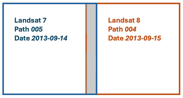
The Roy method for calculating intermission handoffs uses paired images at specific sites, where the reflectance data are obtained from two missions (e.g. Landsat 7 and Landsat 8) separated by one day at a specific location within the overlapping paths in the WRS2 path-row framework:
While Roy et al. (2016) implemented this method on a pixel-by-pixel basis, we implement
using the median band value per site where we have collected data in lakeSR,
available in the lakeSR remote sensing data summary files. This is used in place
of the explicit filters described in the Roy method (saturated pixels,
cloudy/snowy pixels, and pixels with value changes greater than the changes in
atmospheric correction), as we have implemented masks and QA filters to reduce
these sources of error. Handoff coefficients are defined by the ordinary least
squares (OLS) regression line or the Deming regression (minimum likelihood
estimation or MLE, assuming equal and constant error in both x and y variables).
Because Deming regression is computationally intensive, the regression line is
defined by a random sample of 10,000 matches. For the purposes of this
documentation, we only include figures and tables for the Deming regression
(minimum likelihood estimation method) and DSWE1. Intercepts and slopes for all
handoffs are available at the file path
e_calculate_handoffs/out/lakeSR_collated_handoffs_GEEv2025-02-12_QAv2025-06-04.csv
and figures for all handoffs are created when the pipeline is run.
8.3 Gardner method
Gardner method intermission handoffs are defined by the data obtained in the overlapping period of time between two adjacent-in-time missions. These data are filtered to sites that have at least one data point per year for at least 75% of the years of overlap. The filtered data are then summarized to each mission’s 1st-99th percentile value per band, and the handoff coefficients between missions are defined by the second-order polynomial (quadratic) relationship between them. Because this method uses a second-order polynomial to define the handoff relationship, all input (x) values outside of the 1st and 99th percentile values used to define the intermission handoff should be used with extreme caution.
One additional consideration when using the Gardner method is, even when the
number of observations is high, if there is a difference between total
observations contributing to the quantile summaries, there may be systematic
differences built into the coefficients. An example of possible systematic
differences could be fewer observations from oCONUS locations in Landsat 5 due
to data transmission errors. We did not investigate the differences in number of
images listed in Table 8.4 to determine what, if any,
systematic differences are present between the two missions. We provide the
Gardner method handoffs for continuity with the riverSR product for users who
would like that interoperability. As with the Roy, et al. method, intercepts and
slopes for all handoffs are available at the file path
e_calculate_handoffs/out/lakeSR_collated_handoffs_GEEv2025-02-12_QAv2025-06-04.csv
and figures for all handoffs are created when the pipeline is run.
8.4 Implementing Roy Handoffs
Table 8.1 describes the number of matches contributing to the intermission handoffs using the Roy method. We also include figures of the OLS/MLE relationships and the residuals for the MLE corrections in addition to a table of the coefficients for each DSWE1 MLE handoff.
| Early mission | Late mission | n matches |
|---|---|---|
| Landsat 5 | Landsat 7 | 3,801,943 |
| Landsat 7 | Landsat 8 | 909,806 |
| Band | DSWE type |
Satellite to Correct |
Satellite to Harmonize to |
Intercept | Slope |
Minimum Value in Handoff |
Maximum Value in Handoff |
|---|---|---|---|---|---|---|---|
| med_Blue | DSWE1 | LS5 | LS7 | 0.001 | 0.994 | -0.010 | 0.195 |
| med_Green | 0.004 | 1.025 | -0.005 | 0.199 | |||
| med_Red | 0.005 | 0.984 | -0.009 | 0.200 | |||
| med_Nir | 0.002 | 1.016 | -0.008 | 0.200 | |||
| med_Swir1 | -0.002 | 1.360 | -0.006 | 0.098 | |||
| med_Swir2 | -0.001 | 1.360 | -0.007 | 0.082 | |||
| med_SurfaceTemp | -7.348 | 1.027 | 273.150 | 313.150 | |||
| med_Blue | LS8 | -0.010 | 0.768 | -0.008 | 0.195 | ||
| med_Green | -0.009 | 0.991 | -0.006 | 0.200 | |||
| med_Red | -0.009 | 0.967 | -0.008 | 0.200 | |||
| med_Nir | -0.013 | 0.985 | -0.010 | 0.200 | |||
| med_Swir1 | -0.001 | 0.796 | -0.005 | 0.095 | |||
| med_Swir2 | 0.001 | 0.765 | -0.006 | 0.082 | |||
| med_SurfaceTemp | -18.088 | 1.068 | 273.150 | 313.030 | |||
| med_Blue | DSWE1a | LS5 | 0.002 | 0.971 | -0.010 | 0.195 | |
| med_Green | 0.004 | 1.013 | -0.005 | 0.199 | |||
| med_Red | 0.005 | 0.962 | -0.009 | 0.200 | |||
| med_Nir | 0.003 | 0.988 | -0.008 | 0.200 | |||
| med_Swir1 | -0.001 | 1.253 | -0.006 | 0.099 | |||
| med_Swir2 | 0.000 | 1.172 | -0.007 | 0.082 | |||
| med_SurfaceTemp | -7.373 | 1.027 | 273.150 | 313.150 | |||
| med_Blue | LS8 | -0.009 | 0.736 | -0.008 | 0.195 | ||
| med_Green | -0.009 | 0.994 | -0.006 | 0.200 | |||
| med_Red | -0.008 | 0.962 | -0.008 | 0.200 | |||
| med_Nir | -0.017 | 1.112 | -0.010 | 0.200 | |||
| med_Swir1 | 0.000 | 0.774 | -0.005 | 0.098 | |||
| med_Swir2 | 0.001 | 0.719 | -0.006 | 0.082 | |||
| med_SurfaceTemp | -21.097 | 1.078 | 273.150 | 313.030 |
| Band | DSWE type |
Satellite to Correct |
Satellite to Harmonize to |
Intercept | Slope |
Minimum Value in Handoff |
Maximum Value in Handoff |
|---|---|---|---|---|---|---|---|
| med_Blue | DSWE1 | LS7 | LS8 | 0.013 | 1.302 | -0.009 | 0.182 |
| med_Green | 0.009 | 1.009 | 0.000 | 0.199 | |||
| med_Red | 0.009 | 1.034 | -0.010 | 0.200 | |||
| med_Nir | 0.013 | 1.015 | -0.010 | 0.199 | |||
| med_Swir1 | 0.001 | 1.257 | -0.010 | 0.099 | |||
| med_Swir2 | -0.001 | 1.308 | -0.001 | 0.091 | |||
| med_SurfaceTemp | 16.937 | 0.937 | 273.150 | 313.040 | |||
| med_Blue | DSWE1a | 0.012 | 1.359 | -0.010 | 0.182 | ||
| med_Green | 0.009 | 1.006 | 0.000 | 0.199 | |||
| med_Red | 0.009 | 1.040 | -0.010 | 0.200 | |||
| med_Nir | 0.015 | 0.899 | -0.010 | 0.199 | |||
| med_Swir1 | 0.000 | 1.292 | -0.010 | 0.100 | |||
| med_Swir2 | -0.002 | 1.392 | -0.001 | 0.092 | |||
| med_SurfaceTemp | 19.562 | 0.927 | 273.150 | 313.090 |
Application of Roy-style handoffs is straightforward and is completed as simple application of a linear equation:
\[ y = mx + b \]
Where \(b\) is the intercept, \(m\) is the slope, \(x\) is the band reflectance value
from the mission Satellite to Correct in Table 8.2
or 8.3 and \(y\) is the harmonized reflectance value
relative to the mission Satellite to Harmonize to in the previously-mentioned
tables. To reduce output data product size, we do not apply these handoffs
within the output data product, but rather provide users the tools to apply the
handoffs to the filtered lakeSR and siteSR data.
Roy Deming Handoff and Residual Figures
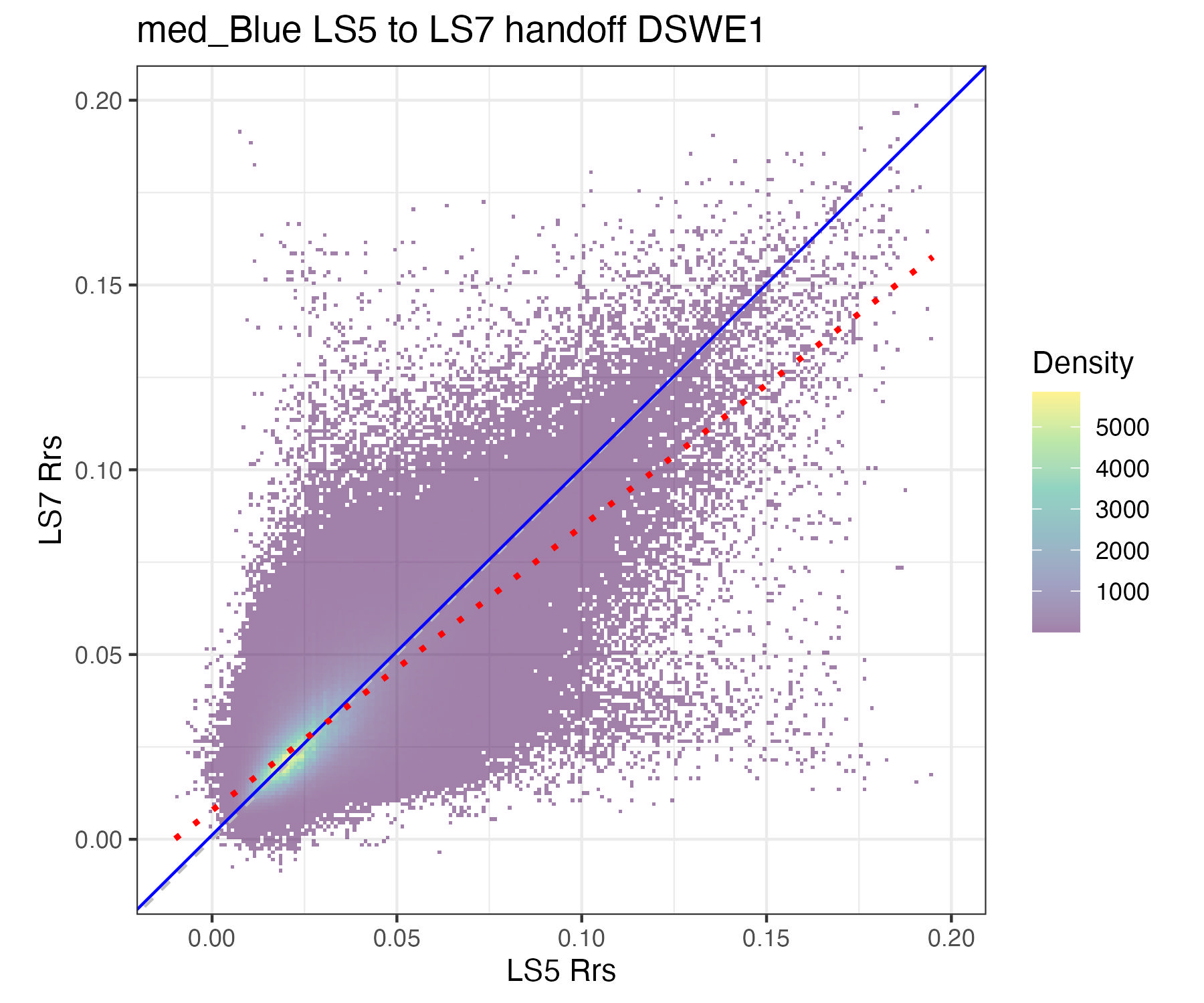
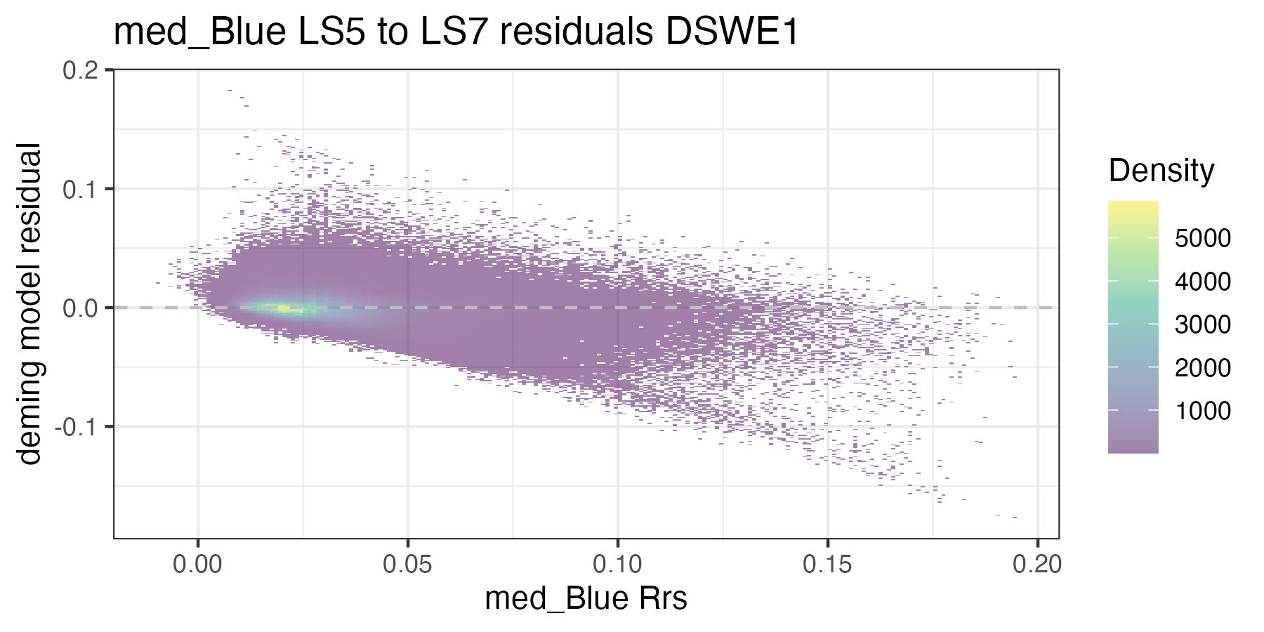
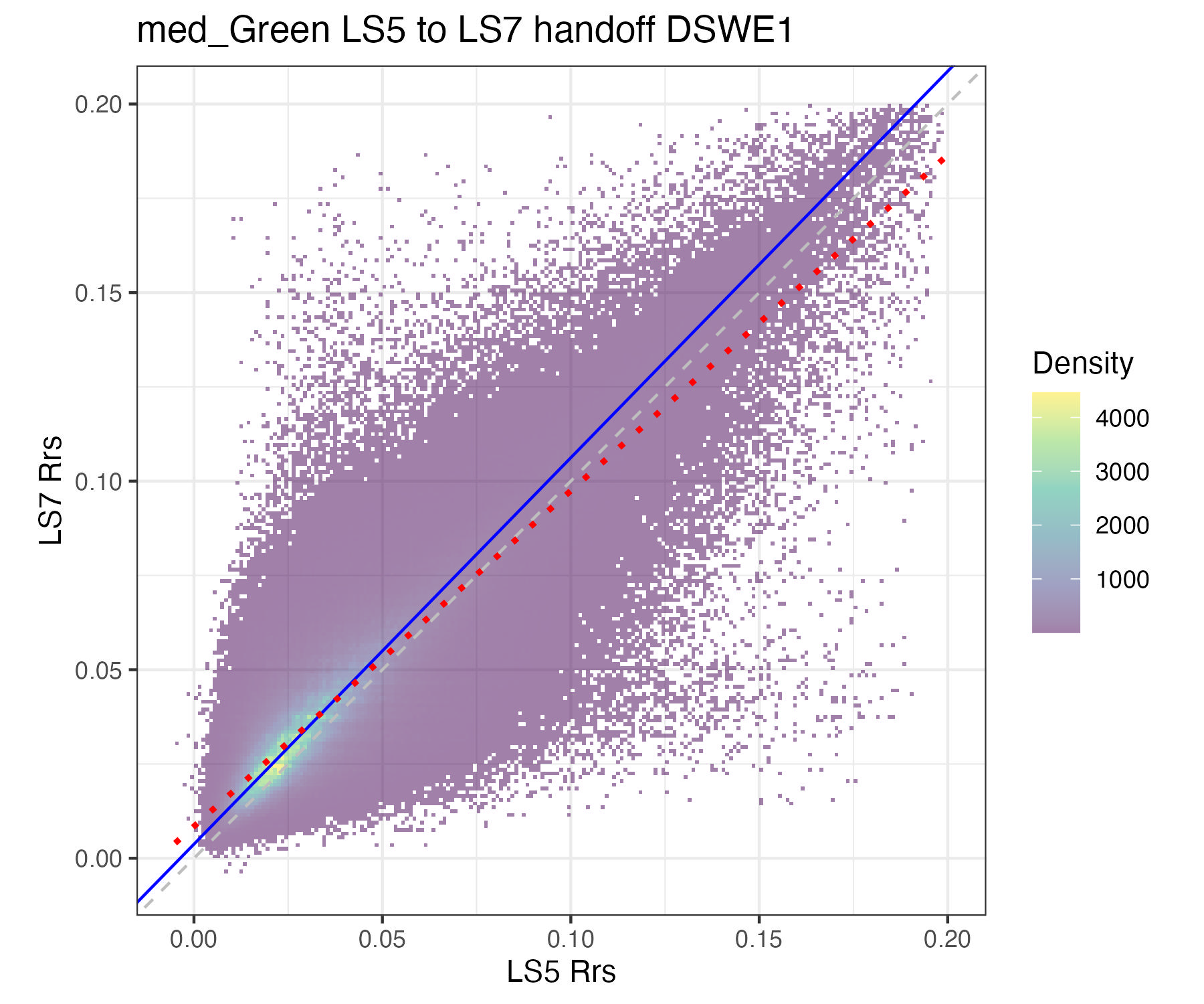
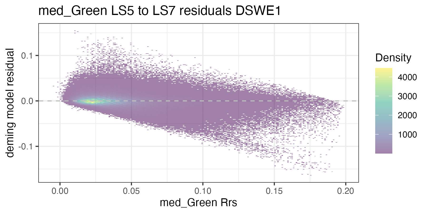
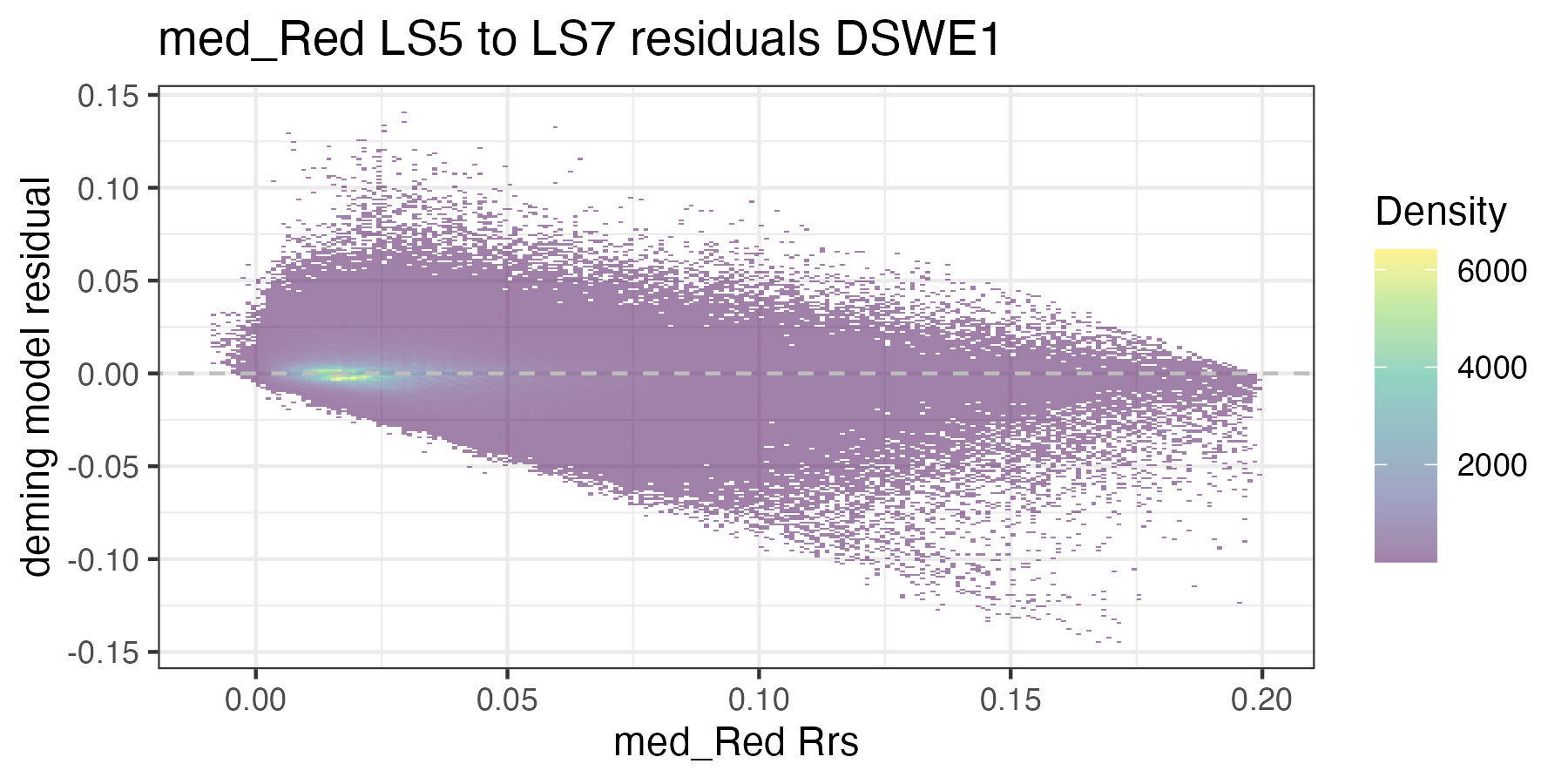
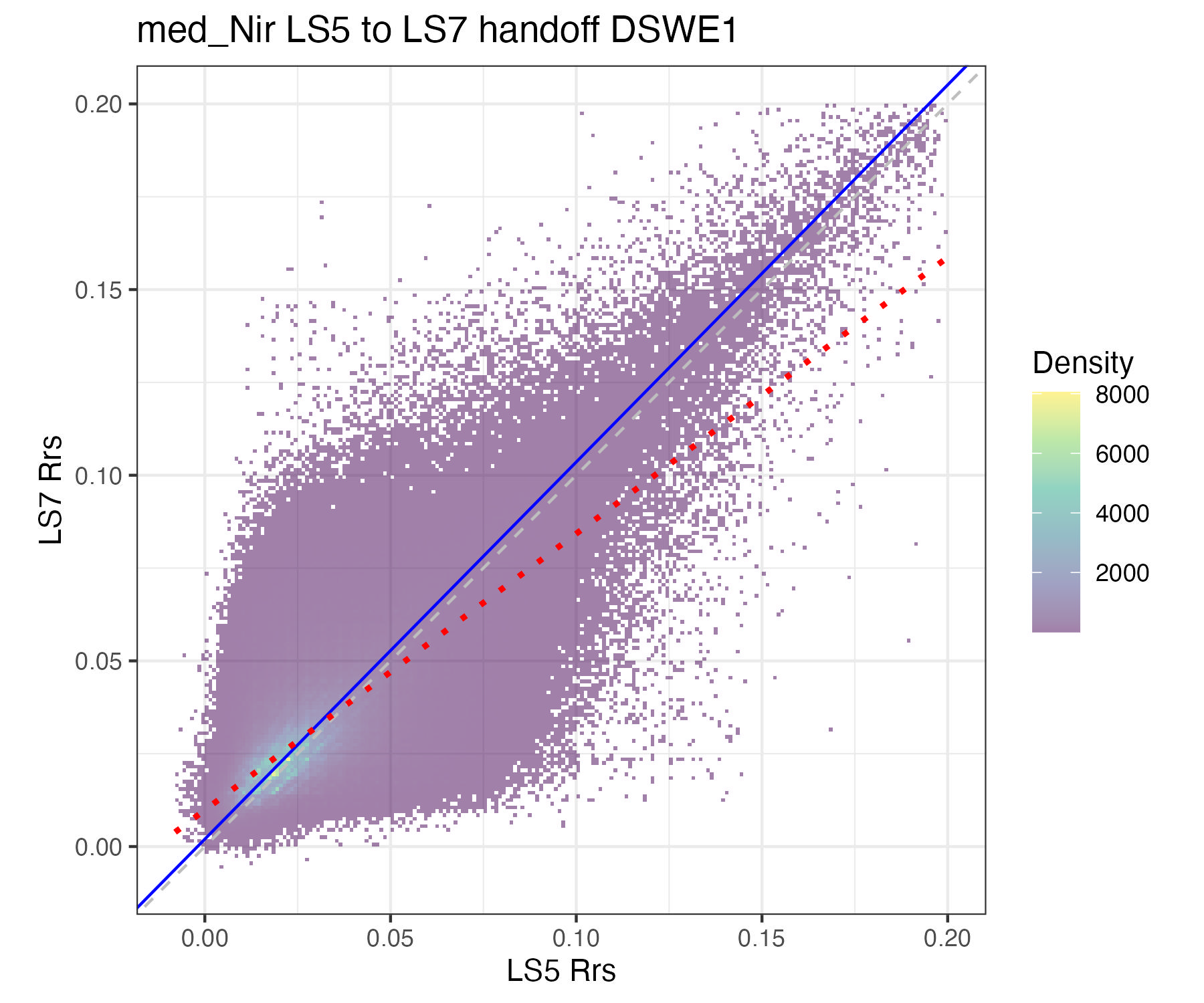
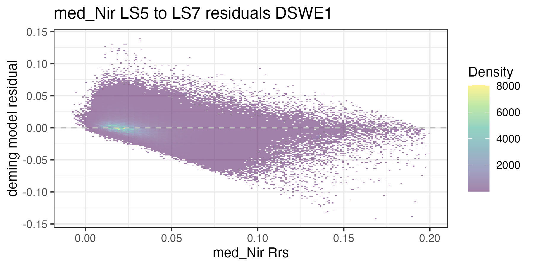
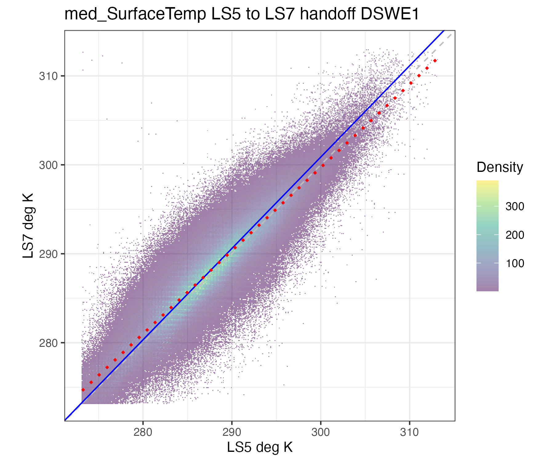
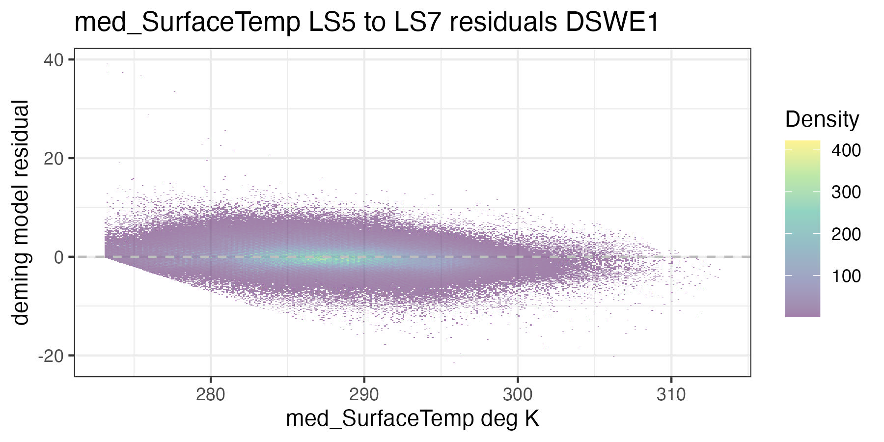
8.4.1 Roy Deming Correction Landsat 5 to Landsat 7
For each of the handoff figures below, the blue line is the Deming (MLE) regression, the red dotted line is the OLS regression line, and the grey dashed line is the 1:1 line. Coefficients for the Deming regression are provided in Table 8.2. Color of dots represents the density of points in at a given x, y location. In the residual plots, the grey dashed line is a 0 intercept, 0 slope line visual aide.
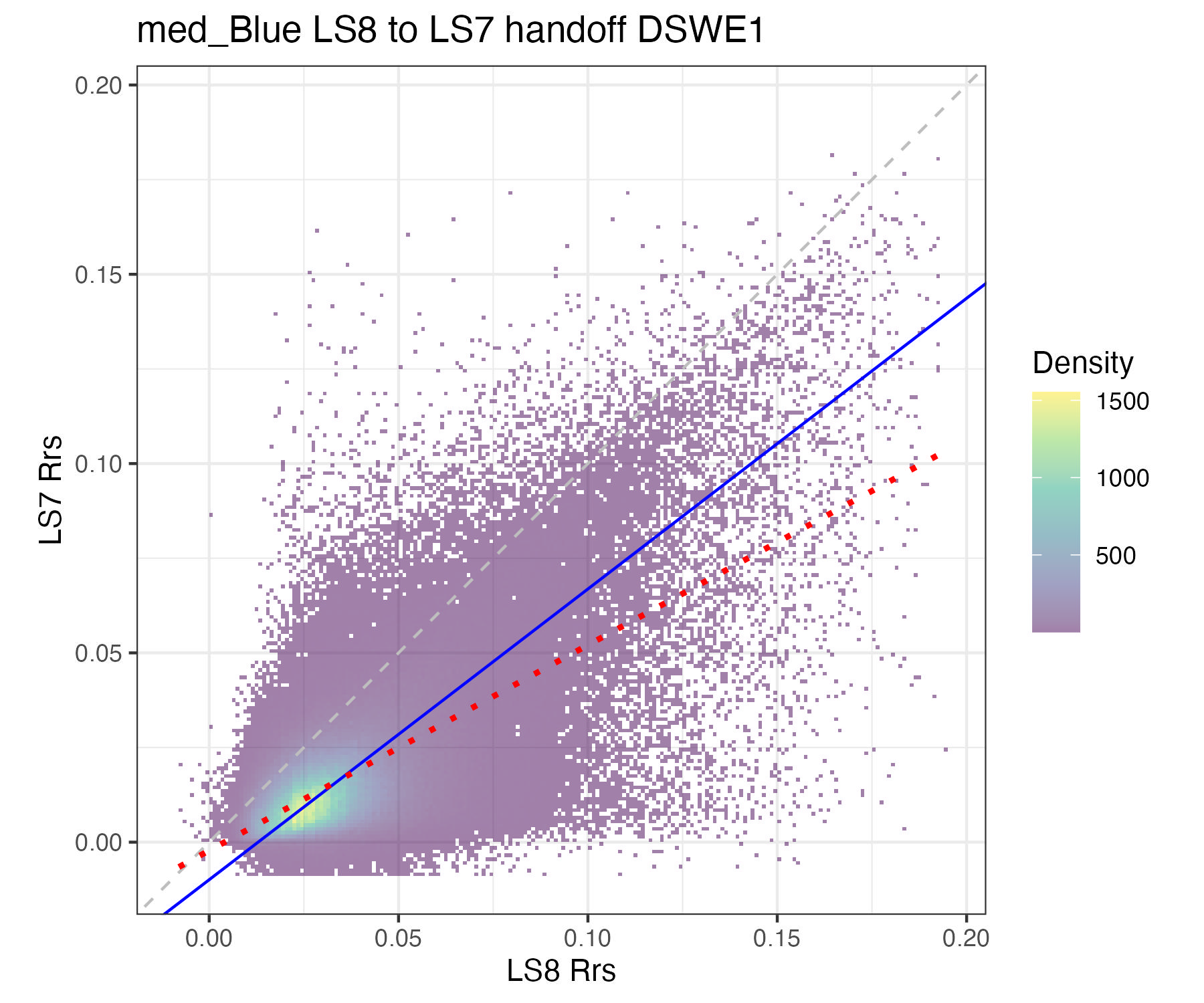
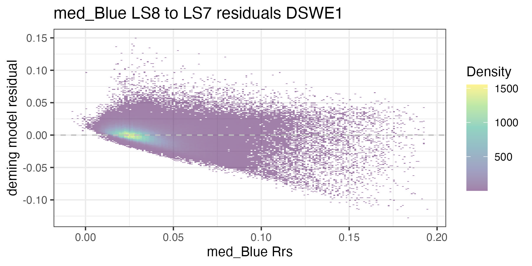
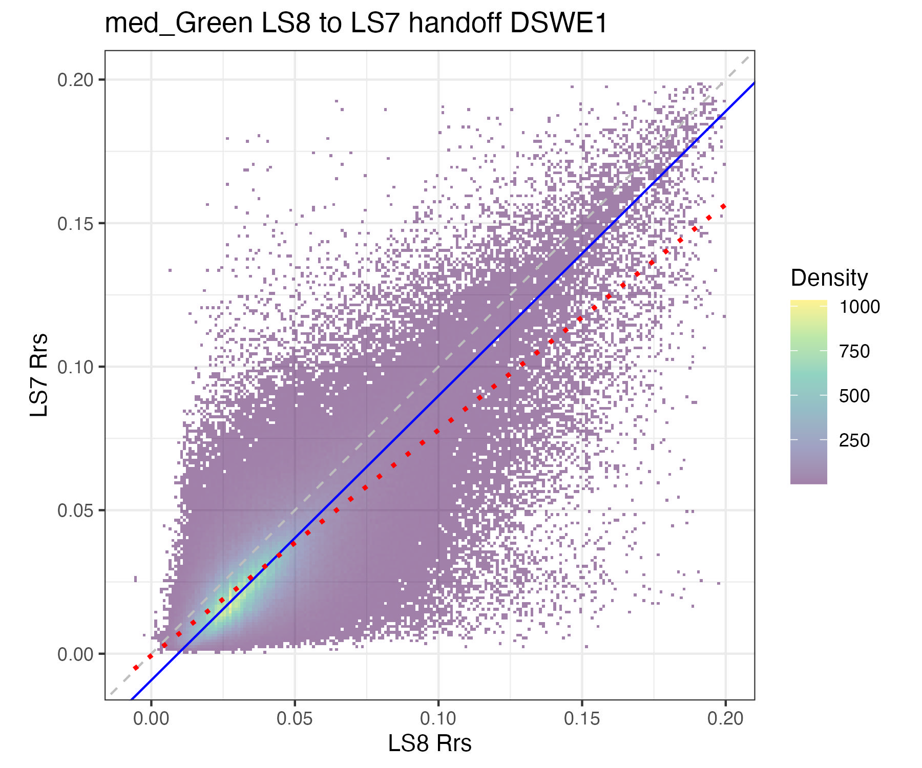
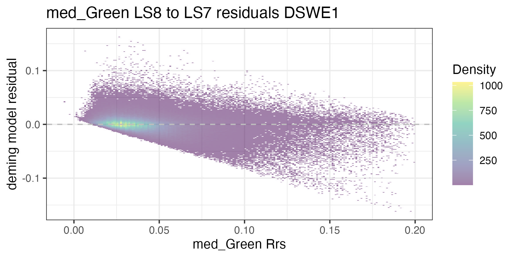
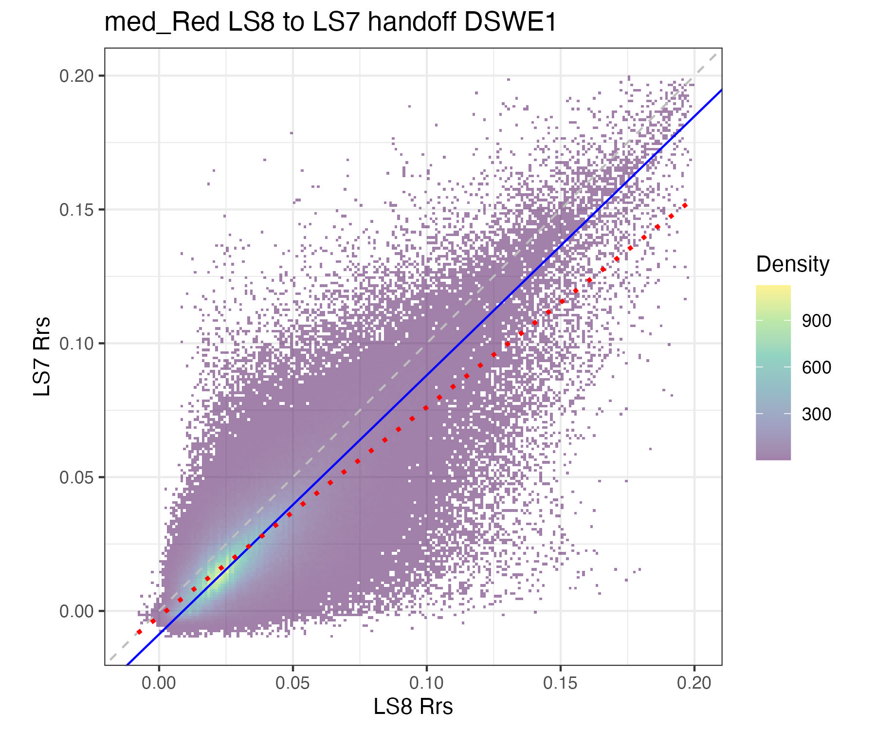
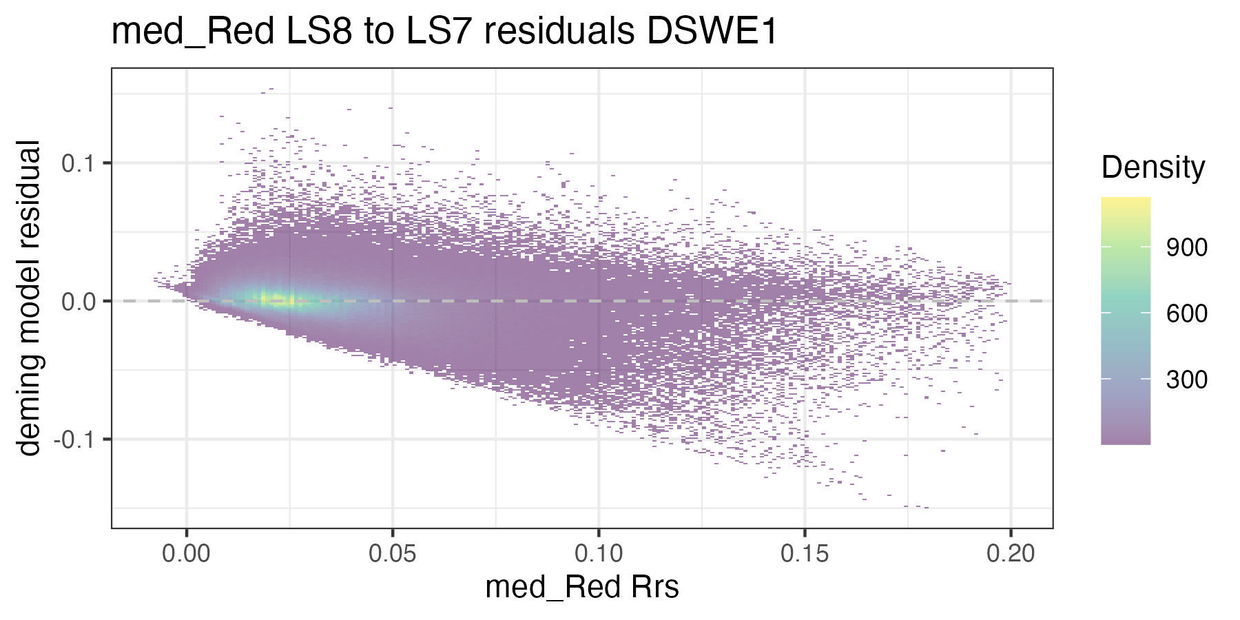
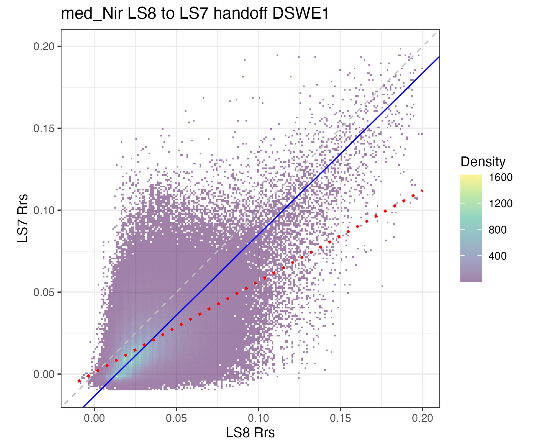
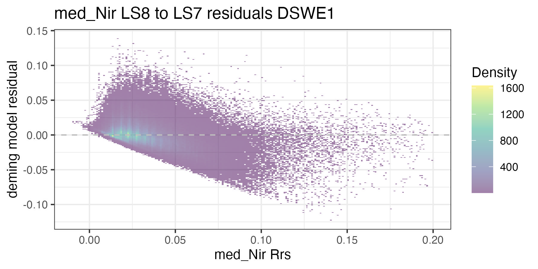
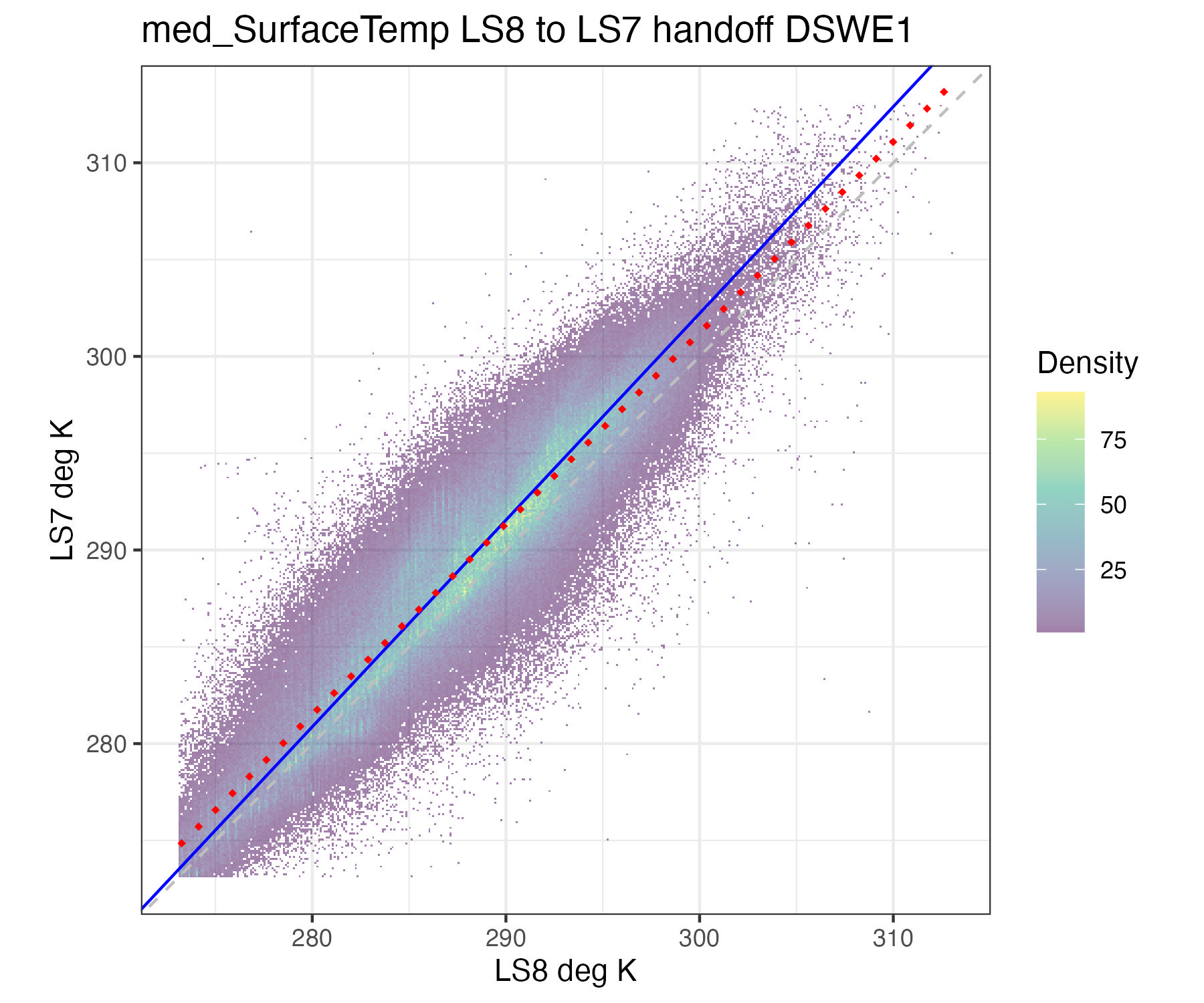
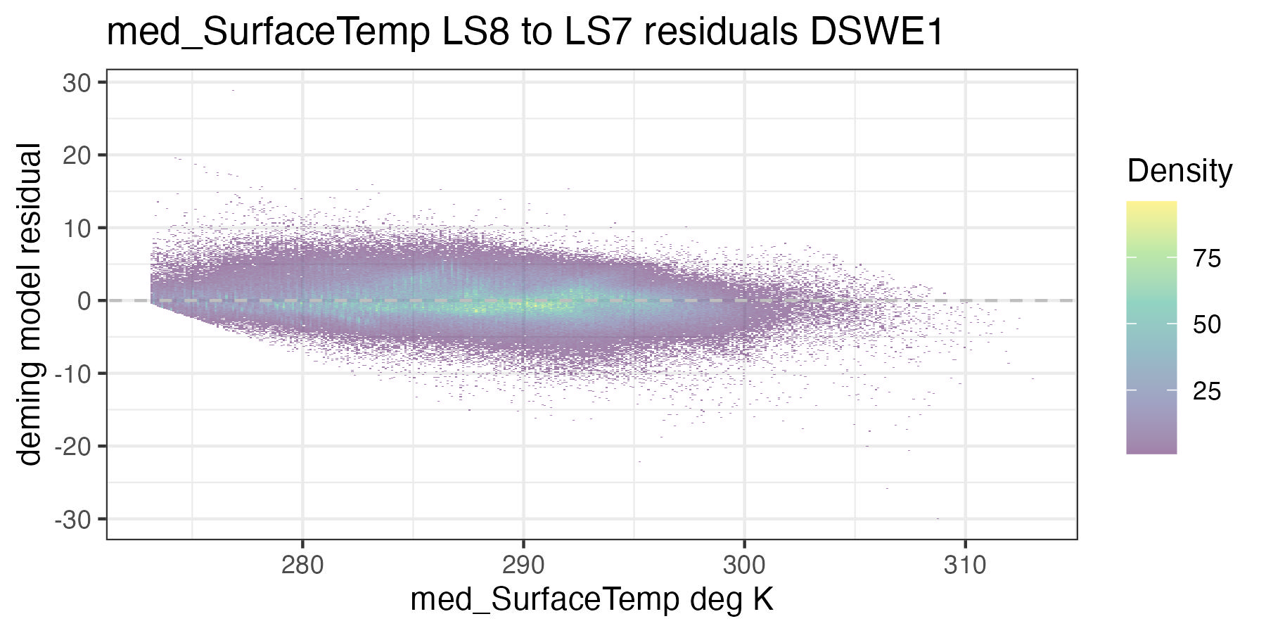
8.4.2 Roy Deming Correction Landsat 8 to Landsat 7
For each of the handoff figures below, the blue solid line is the Deming (MLE) regression, the red line is the OLS regression line, and the grey dashed line is the 1:1 line. Coefficients for the Deming regression are provided in Table 8.2. Color of dots represents the density of points in at a given x, y location. In the residual plots, the grey dashed line is a 0 intercept, 0 slope line visual aide.
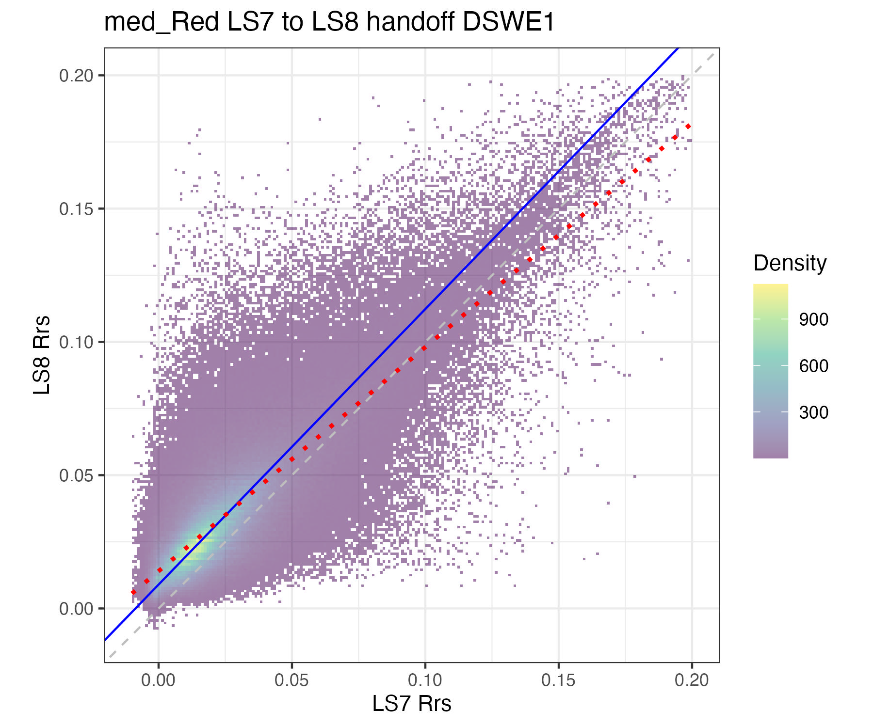
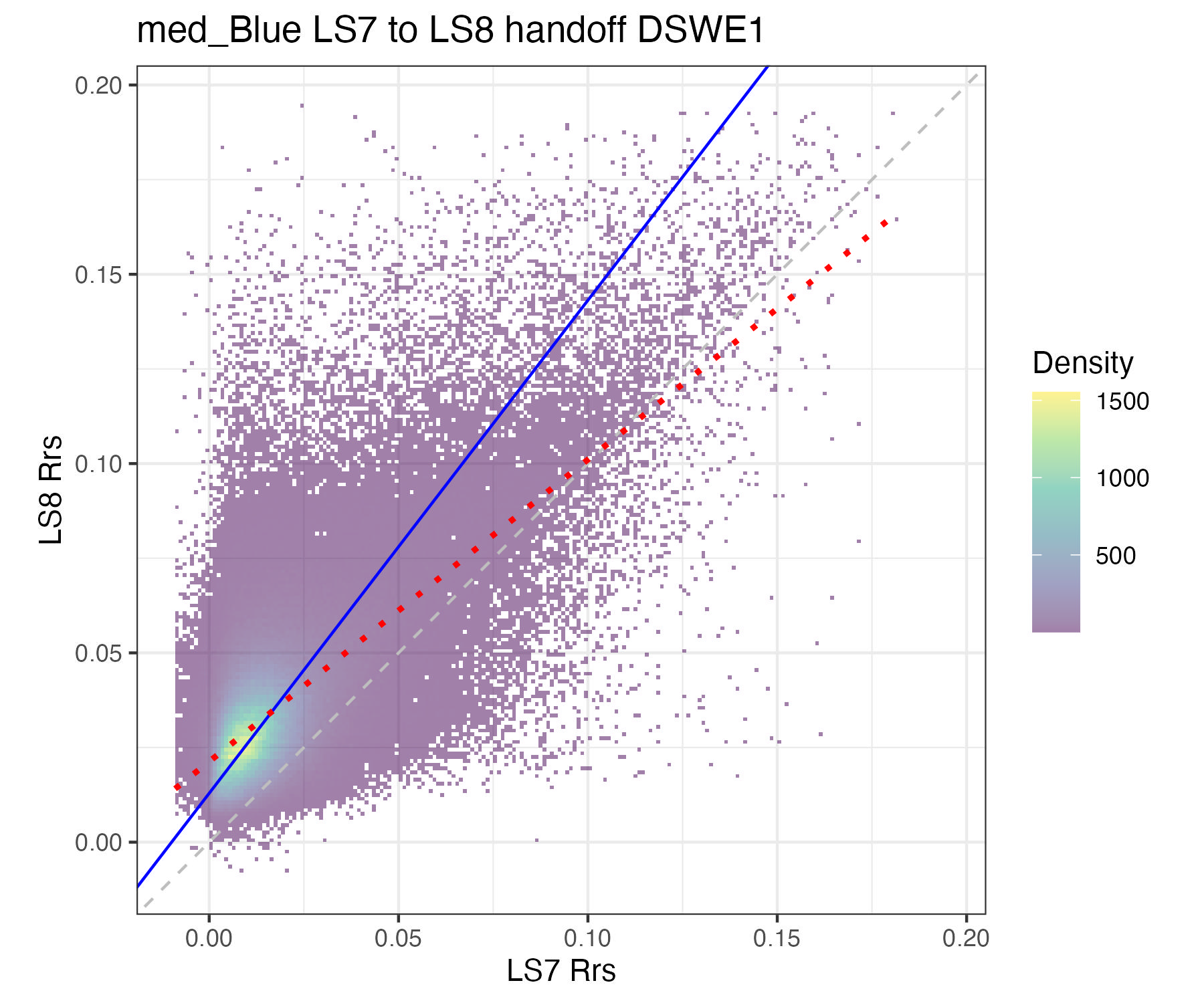
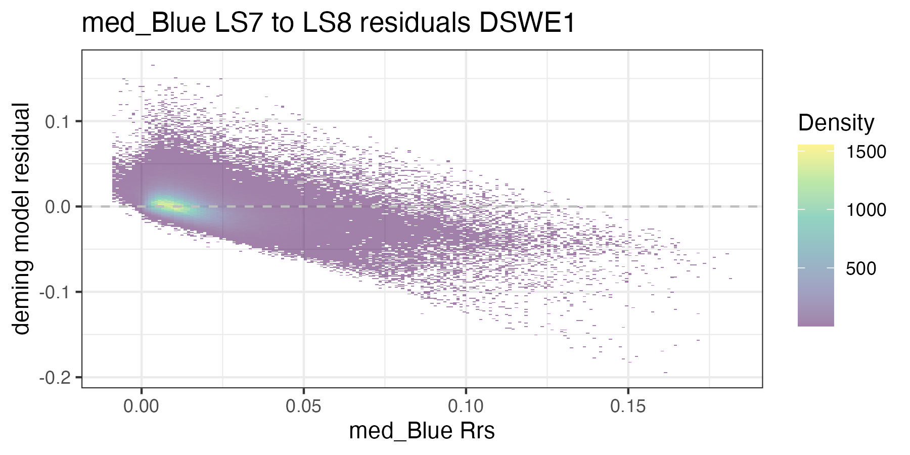
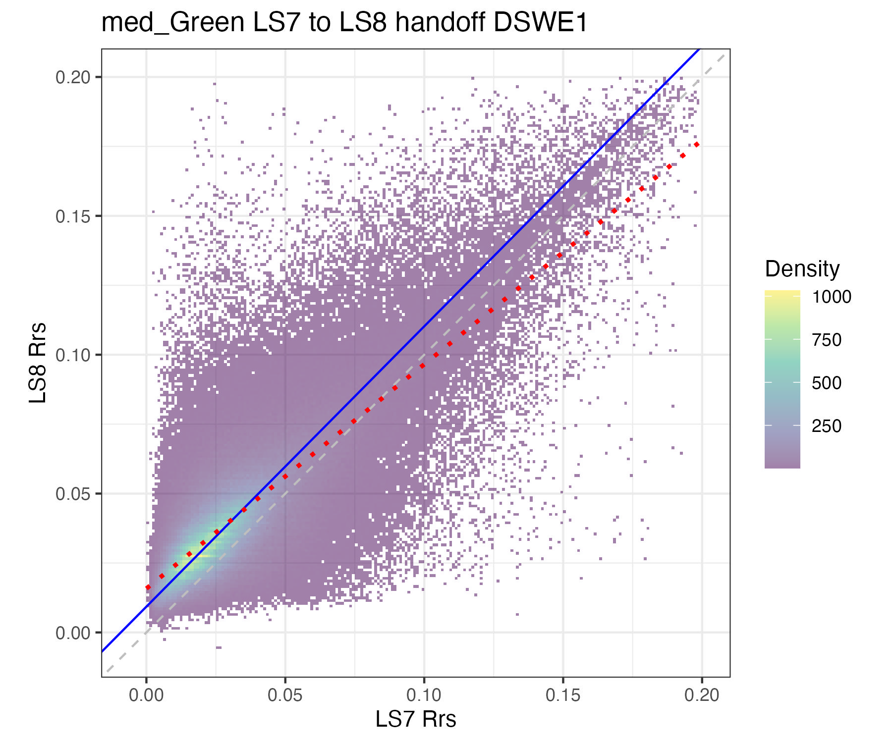
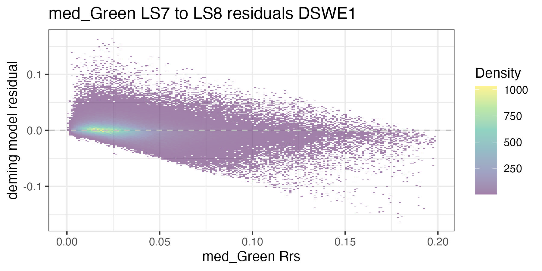
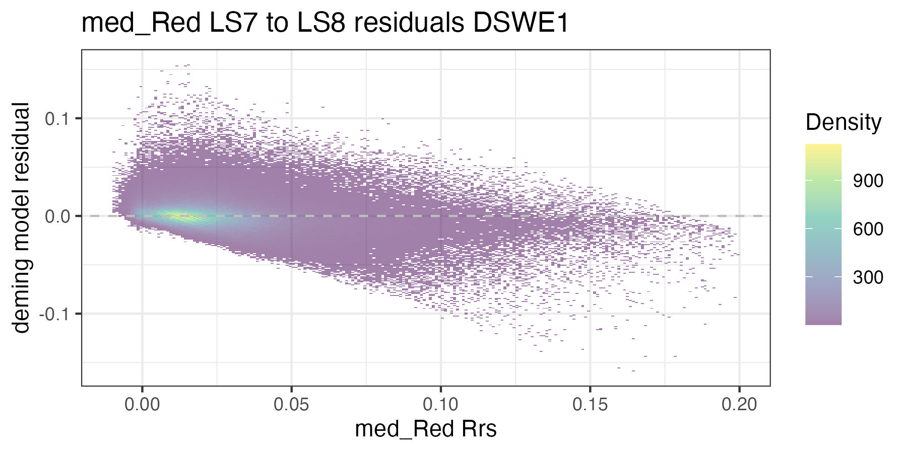
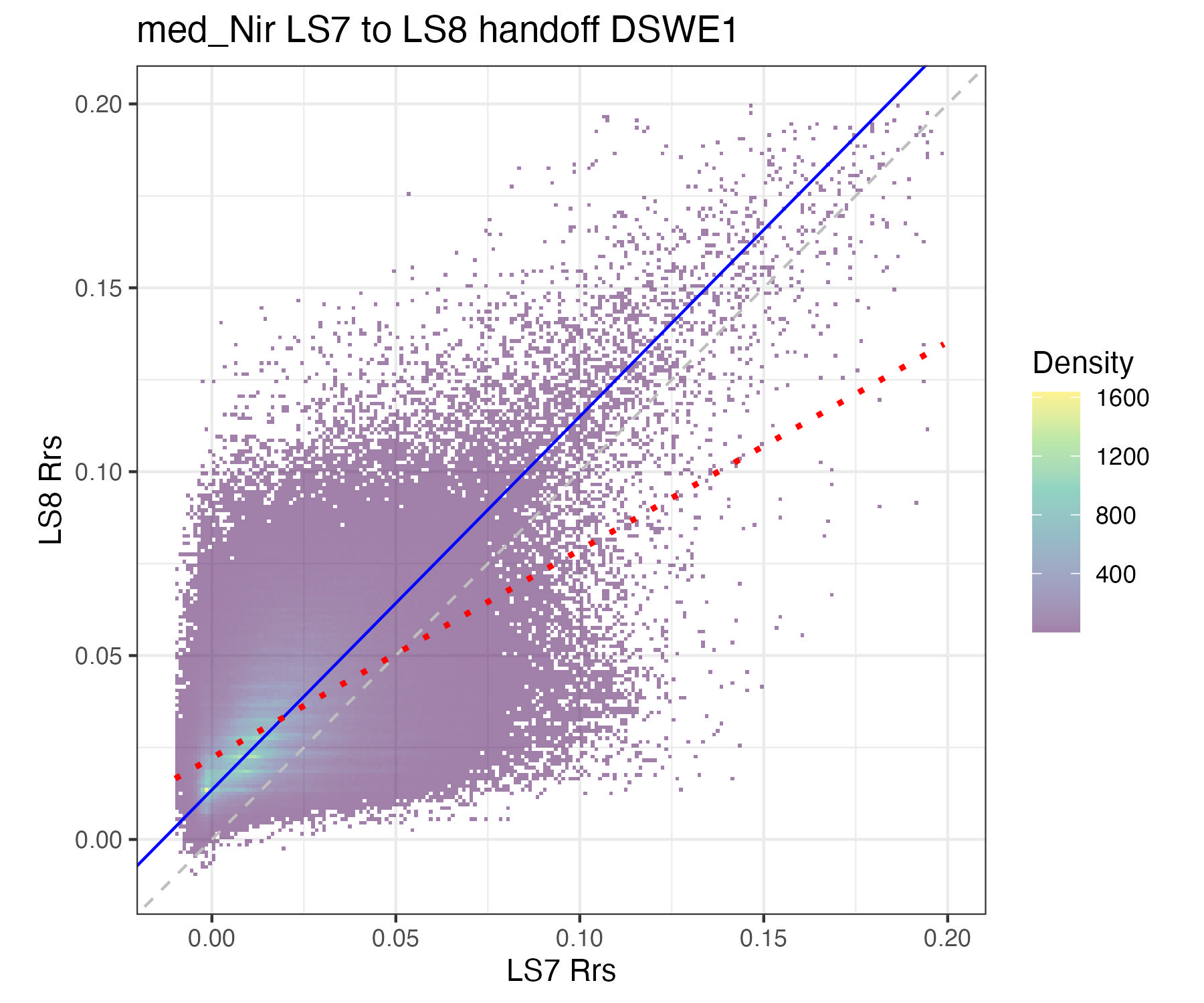
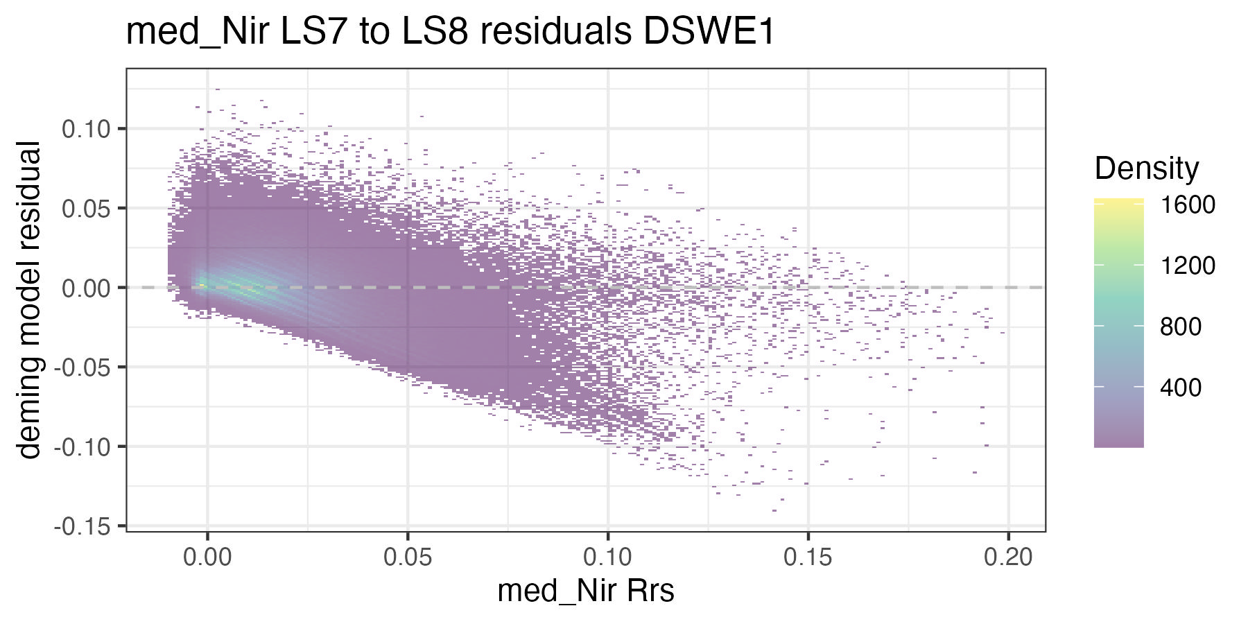
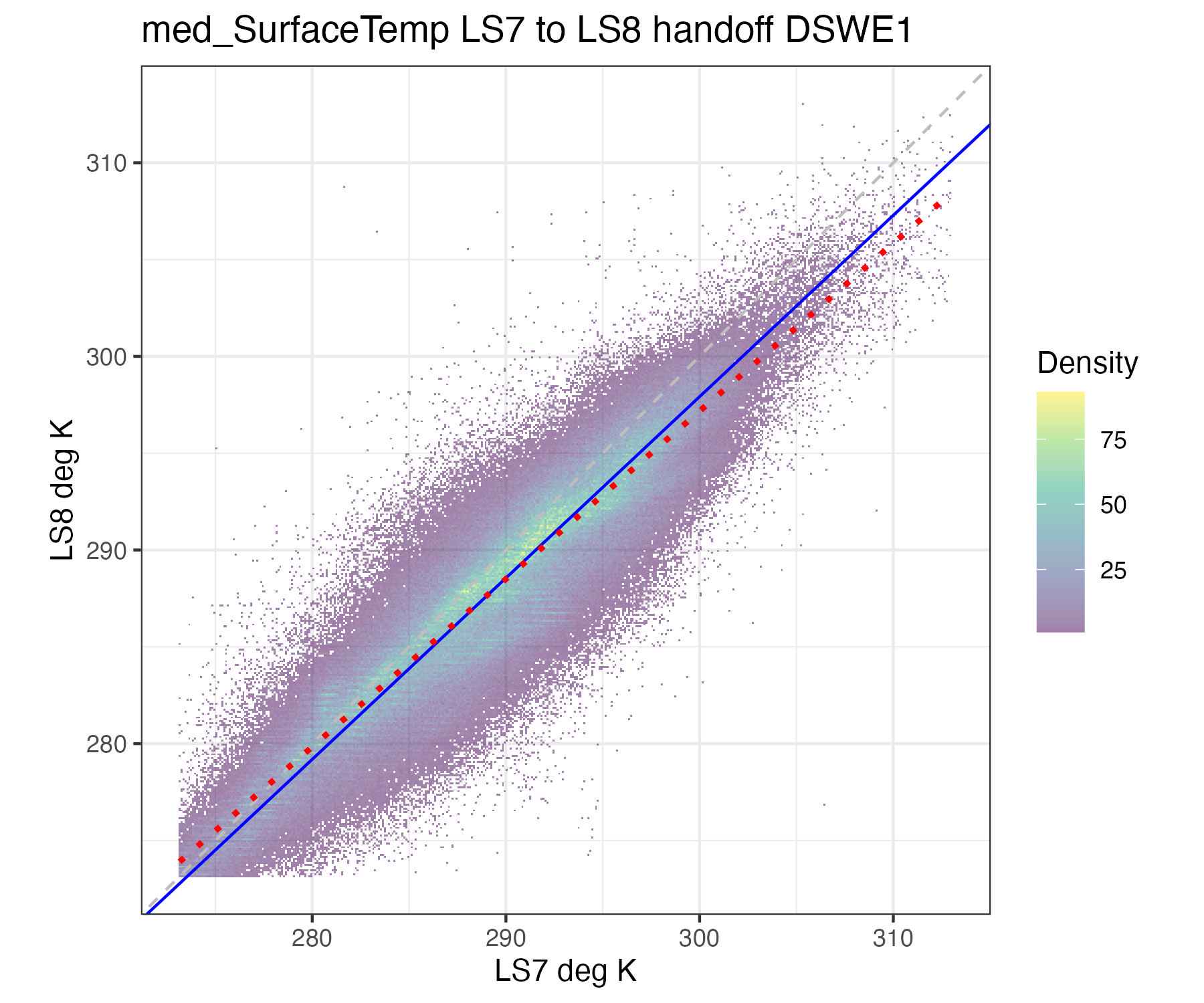
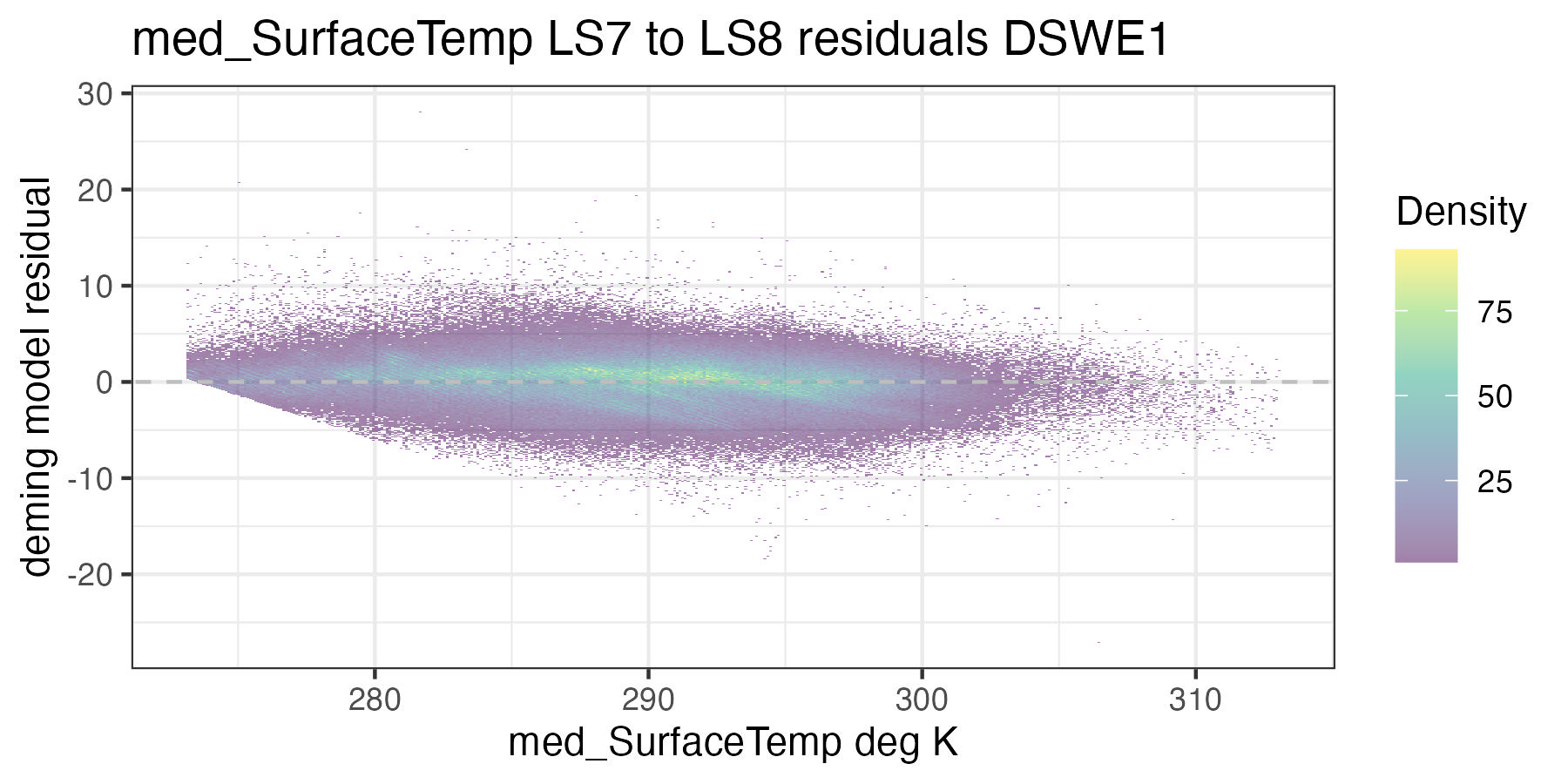
8.4.3 Roy Deming Correction Landsat 7 to Landsat 8
For each of the handoff figures below, the blue solid line is the Deming (MLE) regression, the red dotted line is the OLS regression line, and the grey dashed line is the 1:1 line. Coefficients for the Deming regression are provided in Table 8.3. Color of dots represents the density of points in at a given x, y location. In the residual plots, the grey dashed line is a 0 intercept, 0 slope line visual aide.
8.5 Implementing Gardner Handoffs
| Early mission | Late mission | Correction to | Overlap Start | Overlap End | n Observations from Early Mission | n Observations from Late Mission |
|---|---|---|---|---|---|---|
| Landsat 5 | Landsat 7 | Landsat 7 | 1999-04-15 | 2013-02-11 | 5,645,104 | 13,241,536 |
| Landsat 7 | Landsat 8 | Landsat 7, Landsat8 | 2013-02-11 | 2022-04-16 | 13,655,459 | 2,722,951 |
| Band | DSWE type |
Satellite to Correct |
Satellite to Harmonize to |
Intercept | B1 | B2 |
Minimum Value in Handoff |
Maximum Value in Handoff |
|---|---|---|---|---|---|---|---|---|
| med_Blue | DSWE1 | LS5 | LS7 | 0.005 | 0.681 | 2.054 | 0.010 | 0.097 |
| med_Green | 0.006 | 0.603 | 1.242 | 0.012 | 0.143 | |||
| med_Red | 0.002 | 0.773 | 0.013 | 0.007 | 0.149 | |||
| med_Nir | 0.000 | 0.920 | -1.545 | 0.011 | 0.126 | |||
| med_Swir1 | 0.002 | 0.690 | 2.427 | 0.002 | 0.053 | |||
| med_Swir2 | 0.001 | 0.682 | 3.426 | -0.002 | 0.040 | |||
| med_SurfaceTemp | 245.528 | -0.664 | 0.003 | 274.170 | 304.320 | |||
| med_Blue | LS8 | 0.010 | 1.239 | -3.425 | 0.001 | 0.090 | ||
| med_Green | 0.008 | 0.746 | 1.005 | 0.005 | 0.131 | |||
| med_Red | 0.007 | 0.898 | 0.444 | -0.002 | 0.123 | |||
| med_Nir | 0.013 | 0.733 | 0.513 | -0.003 | 0.099 | |||
| med_Swir1 | 0.003 | 0.928 | -0.284 | 0.000 | 0.047 | |||
| med_Swir2 | 0.001 | 0.971 | -1.414 | 0.001 | 0.037 | |||
| med_SurfaceTemp | 387.600 | -1.604 | 0.004 | 273.890 | 304.540 | |||
| med_Blue | DSWE1a | LS5 | 0.005 | 0.683 | 2.046 | 0.010 | 0.097 | |
| med_Green | 0.006 | 0.605 | 1.218 | 0.012 | 0.143 | |||
| med_Red | 0.002 | 0.780 | -0.018 | 0.007 | 0.149 | |||
| med_Nir | 0.000 | 0.921 | -1.587 | 0.011 | 0.129 | |||
| med_Swir1 | 0.002 | 0.682 | 2.471 | 0.002 | 0.054 | |||
| med_Swir2 | 0.001 | 0.646 | 4.662 | -0.002 | 0.040 | |||
| med_SurfaceTemp | 251.332 | -0.705 | 0.003 | 274.170 | 304.350 | |||
| med_Blue | LS8 | 0.010 | 1.237 | -3.298 | 0.000 | 0.089 | ||
| med_Green | 0.009 | 0.709 | 1.363 | 0.005 | 0.130 | |||
| med_Red | 0.007 | 0.905 | 0.491 | -0.002 | 0.122 | |||
| med_Nir | 0.013 | 0.732 | -0.738 | -0.003 | 0.123 | |||
| med_Swir1 | 0.003 | 0.910 | -1.816 | 0.000 | 0.054 | |||
| med_Swir2 | 0.001 | 0.950 | -2.208 | 0.001 | 0.039 | |||
| med_SurfaceTemp | 430.713 | -1.903 | 0.005 | 273.910 | 304.570 |
| Band | DSWE type |
Satellite to Correct |
Satellite to Harmonize to |
Intercept | B1 | B2 |
Minimum Value in Handoff |
Maximum Value in Handoff |
|---|---|---|---|---|---|---|---|---|
| med_Blue | DSWE1 | LS7 | LS8 | -0.007 | 0.651 | 3.909 | 0.010 | 0.095 |
| med_Green | -0.011 | 1.332 | -1.498 | 0.011 | 0.123 | |||
| med_Red | -0.007 | 1.111 | -0.475 | 0.005 | 0.123 | |||
| med_Nir | -0.018 | 1.375 | -0.966 | 0.008 | 0.093 | |||
| med_Swir1 | -0.003 | 1.057 | 0.740 | 0.002 | 0.046 | |||
| med_Swir2 | -0.001 | 0.987 | 2.804 | 0.000 | 0.035 | |||
| med_SurfaceTemp | -511.883 | 4.481 | -0.006 | 273.720 | 301.330 | |||
| med_Blue | DSWE1a | -0.007 | 0.667 | 3.629 | 0.010 | 0.095 | ||
| med_Green | -0.011 | 1.383 | -1.989 | 0.011 | 0.123 | |||
| med_Red | -0.007 | 1.101 | -0.498 | 0.005 | 0.123 | |||
| med_Nir | -0.017 | 1.272 | 2.616 | 0.008 | 0.095 | |||
| med_Swir1 | -0.003 | 1.049 | 3.592 | 0.002 | 0.047 | |||
| med_Swir2 | -0.001 | 1.003 | 4.277 | 0.000 | 0.035 | |||
| med_SurfaceTemp | -567.756 | 4.872 | -0.007 | 273.720 | 301.380 |
Application of Gardner-style handoffs is completed as simple application of a second order polynomial equation:
\[ y = b0 + b1*x + b2*x^2 \]
Where \(b0\) is the intercept, \(b1\) is the coefficient of the \(x\) value, \(b2\) is
the coefficient of the quadratic term \(x^2\), \(x\) is the band reflectance value
from the mission Satellite to Correct in Table 8.5 or
8.6 and \(y\) is the harmonized reflectance value relative
to the mission Satellite to Harmonize to in the previously-mentioned tables.
To reduce output data product size, we do not apply these handoffs within the
output data product, but rather provide users the tools to apply the handoffs to
the filtered lakeSR and siteSR data.
Gardner Handoff and Residual Figures relative to Landsat 7
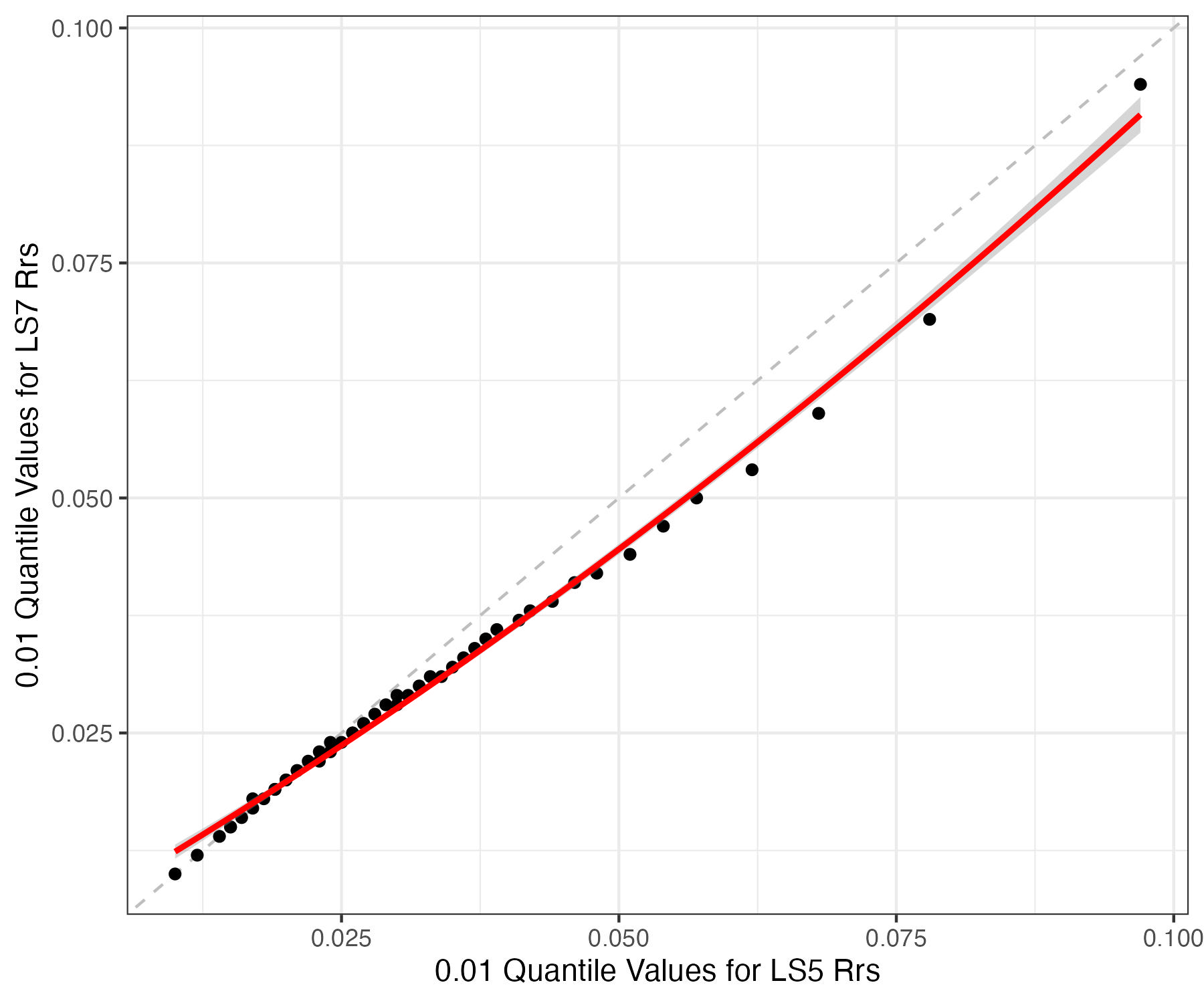
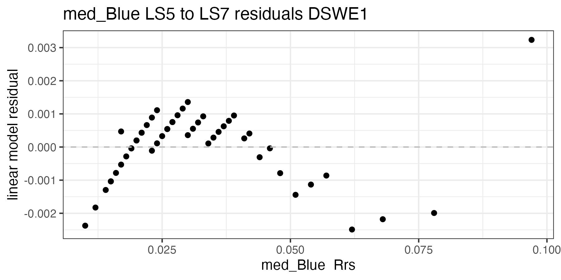
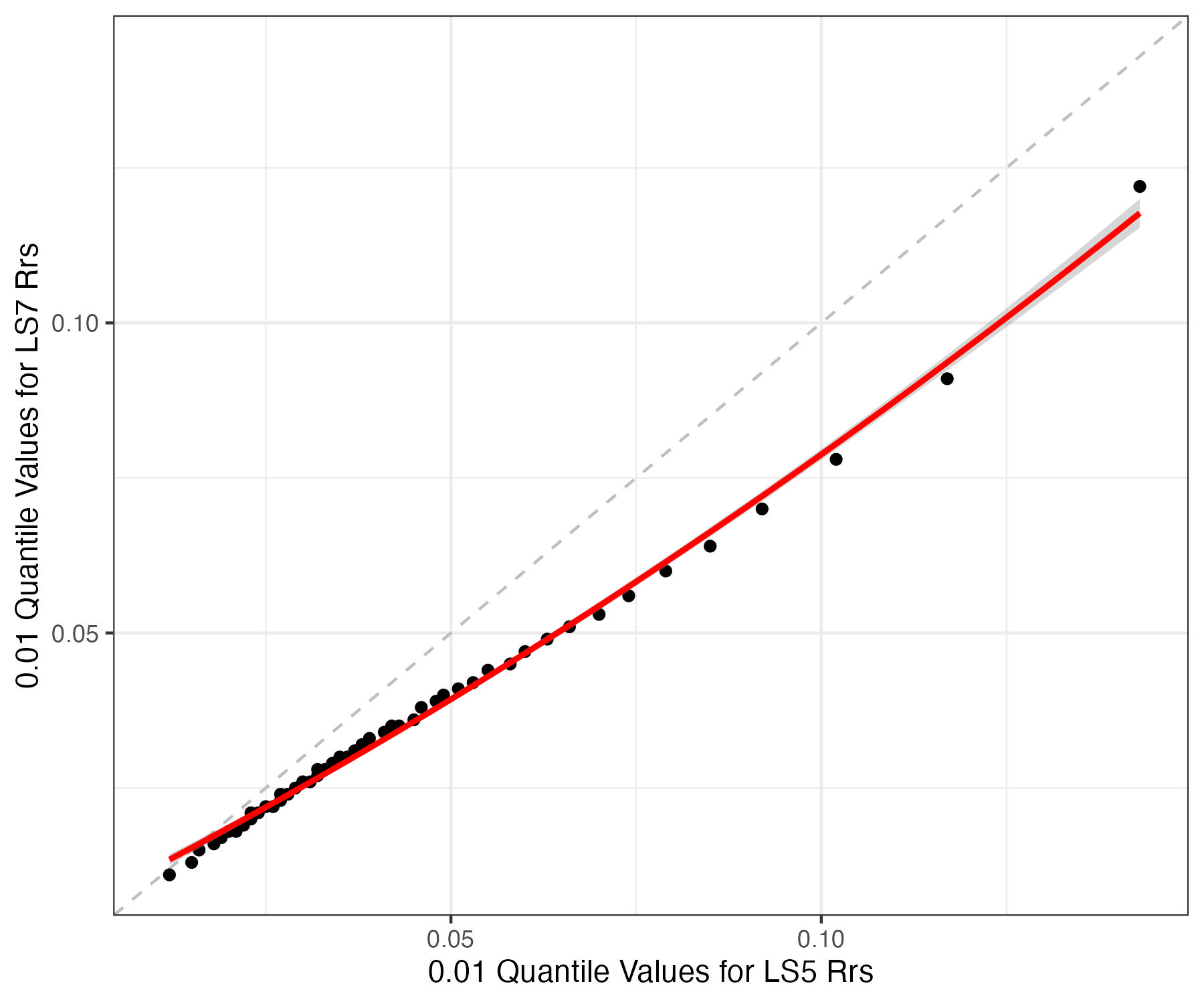
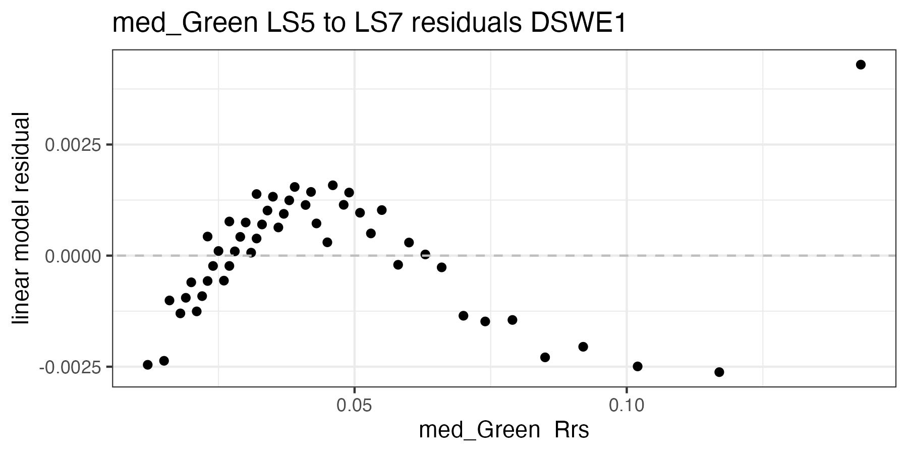
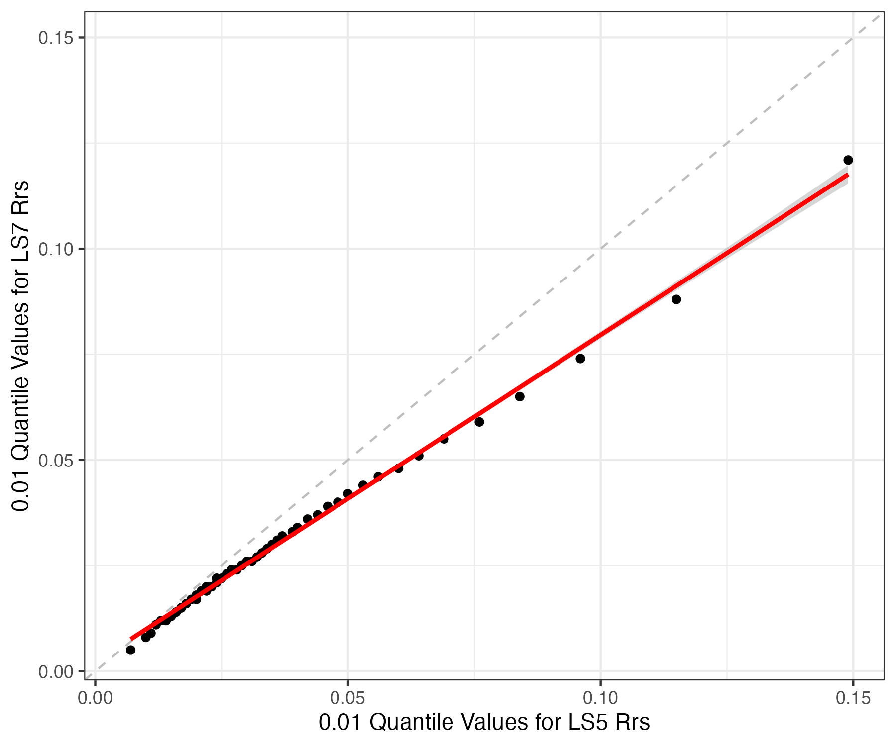
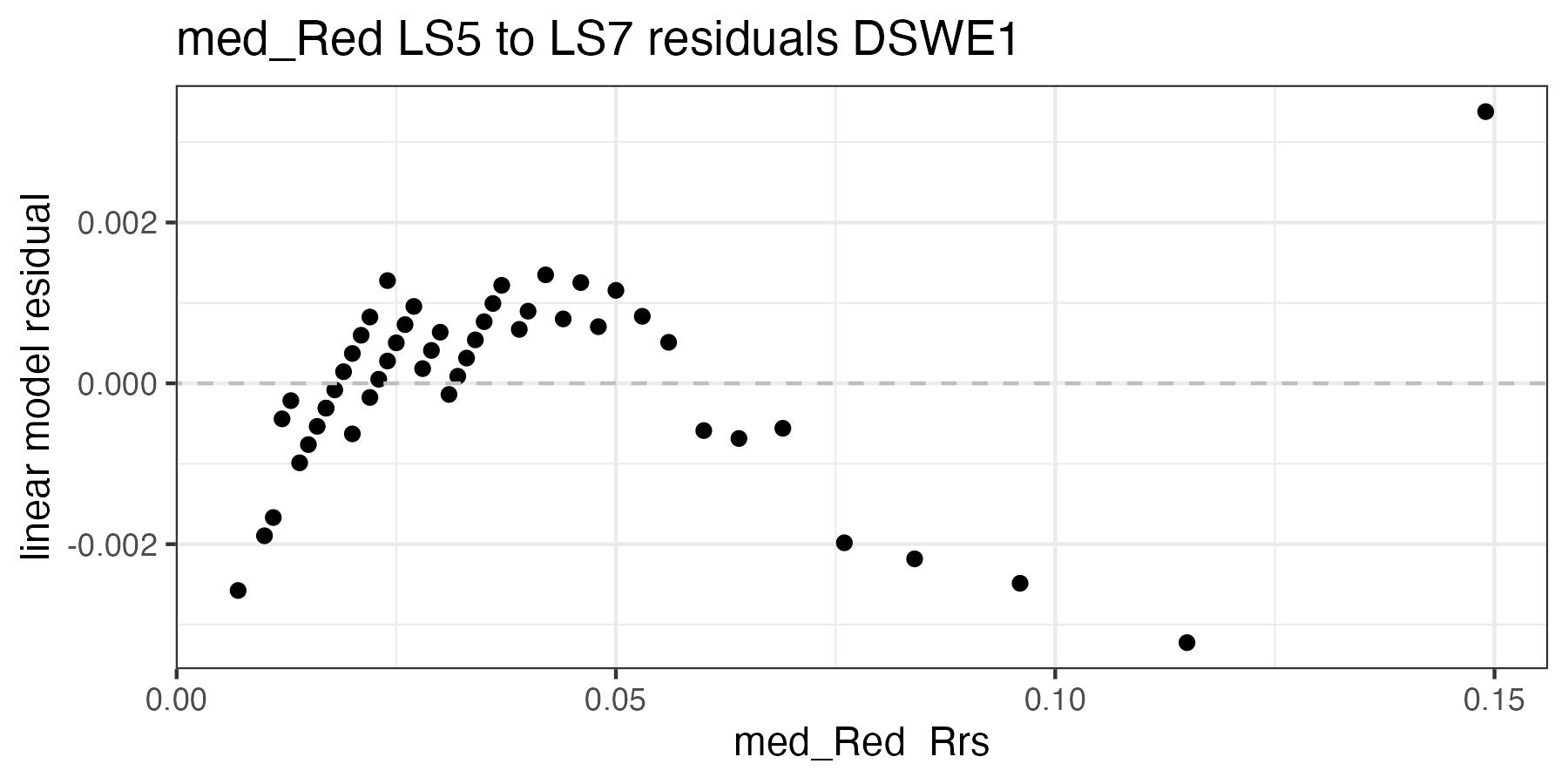
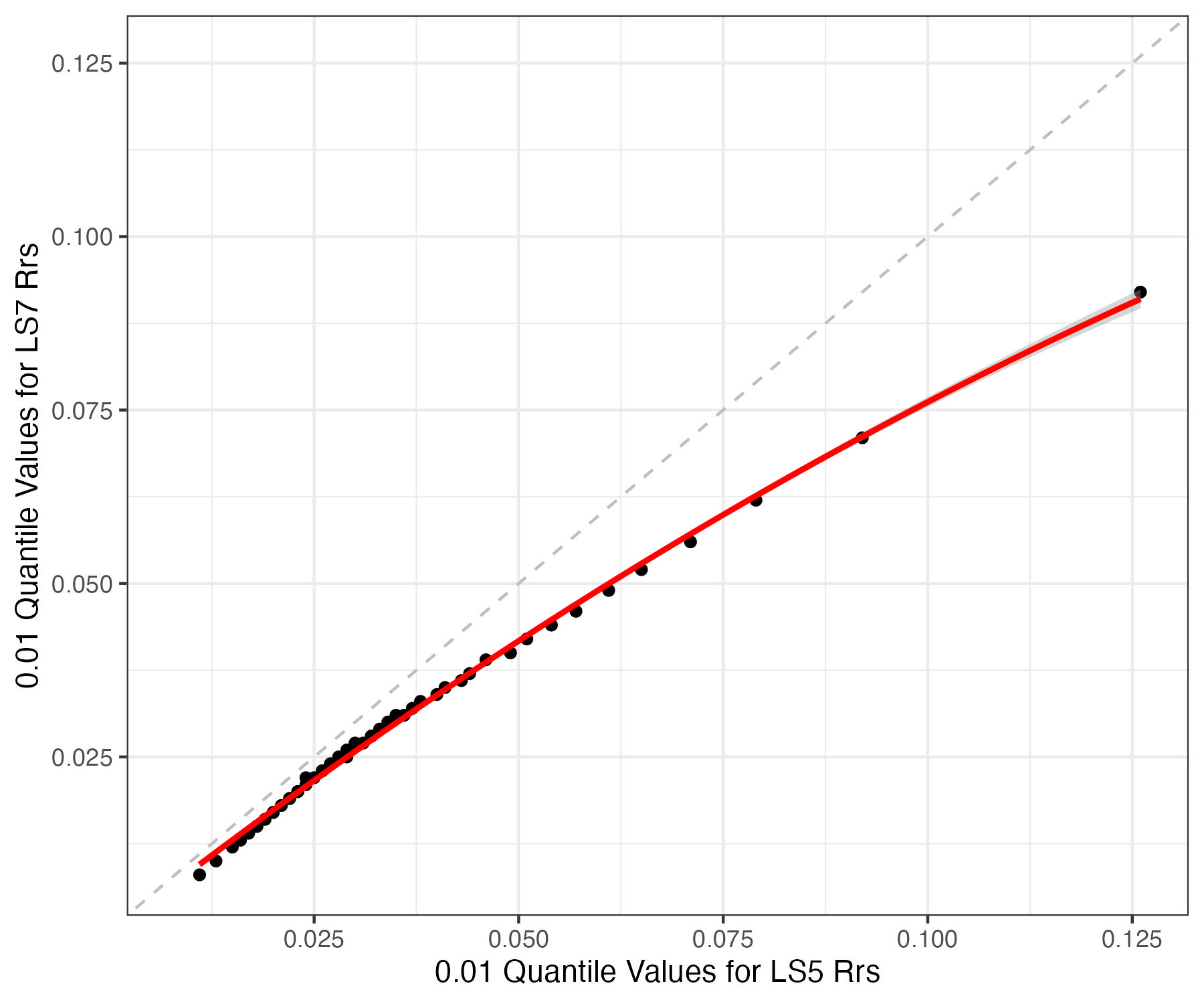
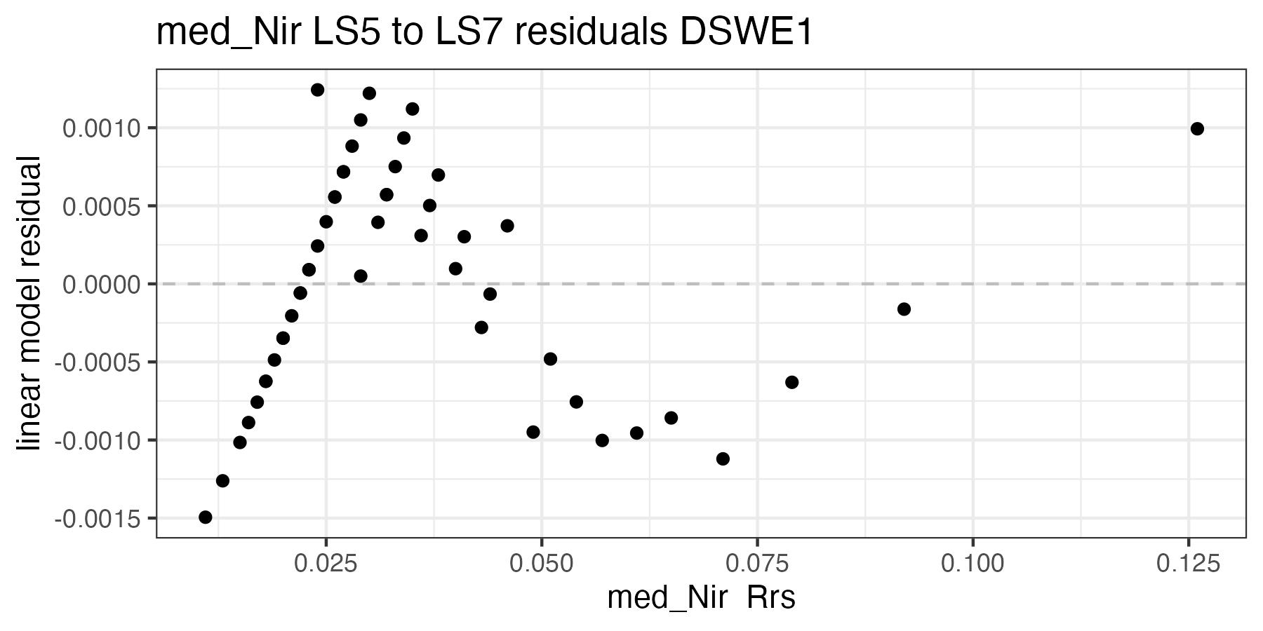
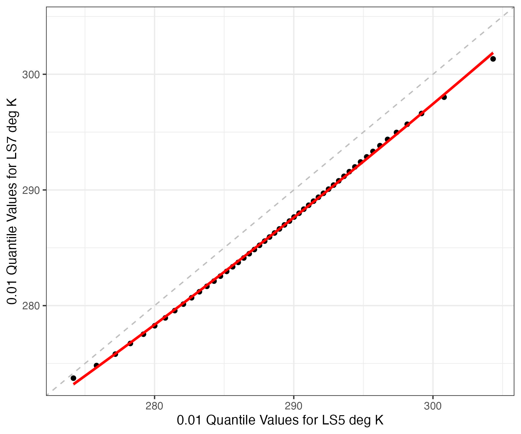
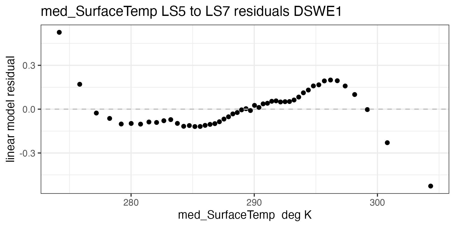
8.5.1 Gardner Correction Landsat 5 to Landsat 7
For each of the handoff figures below, the red line is the second order polynomial regression and the grey dashed line is the 1:1 line. Coefficients for the second order polynomial regression are provided in Table 8.5. Color of dots represents the density of points in at a given x, y location. In the residual plots, the grey dashed line is a 0 intercept, 0 slope line visual aide.
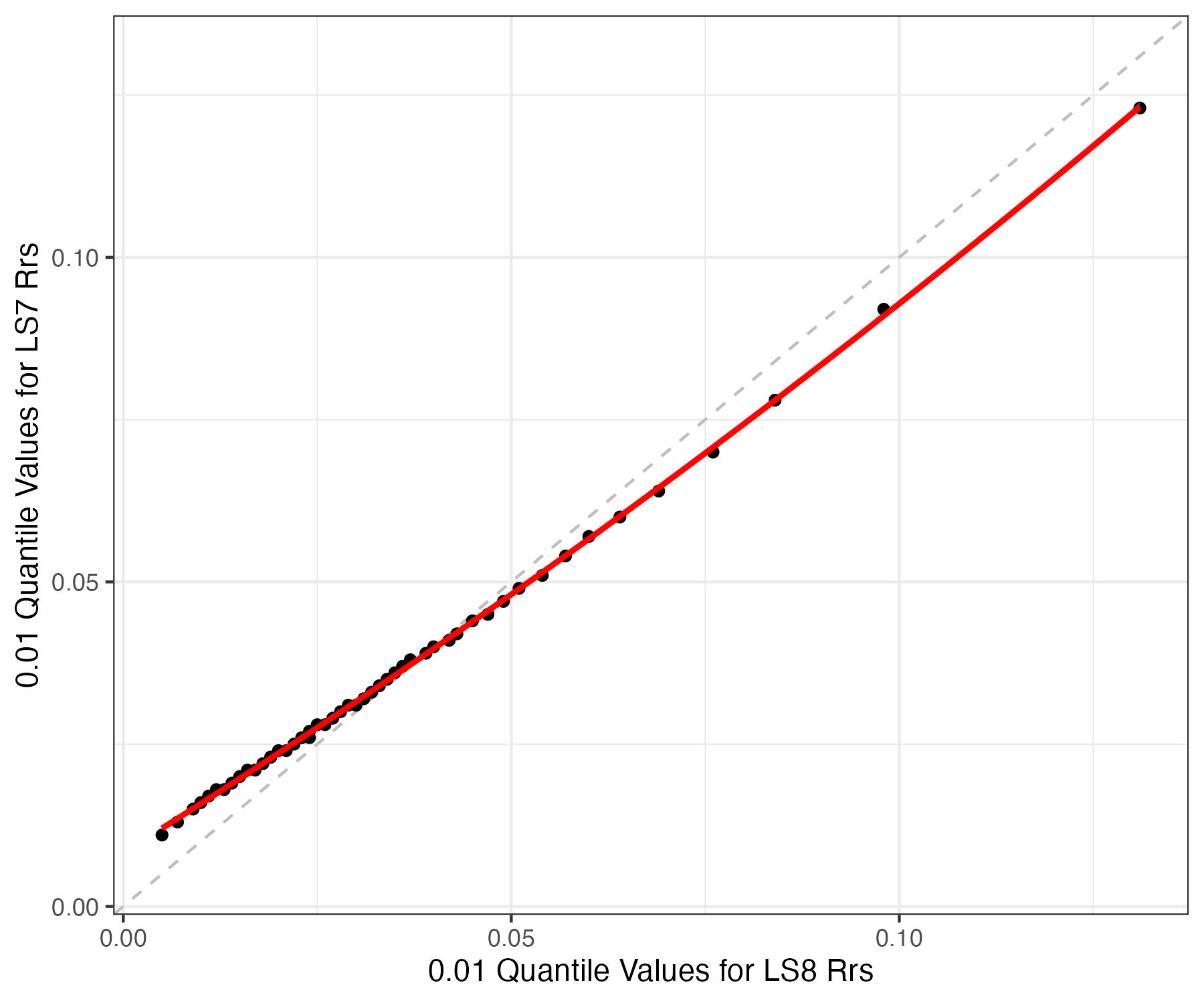
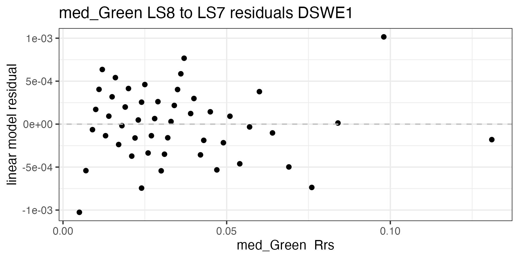
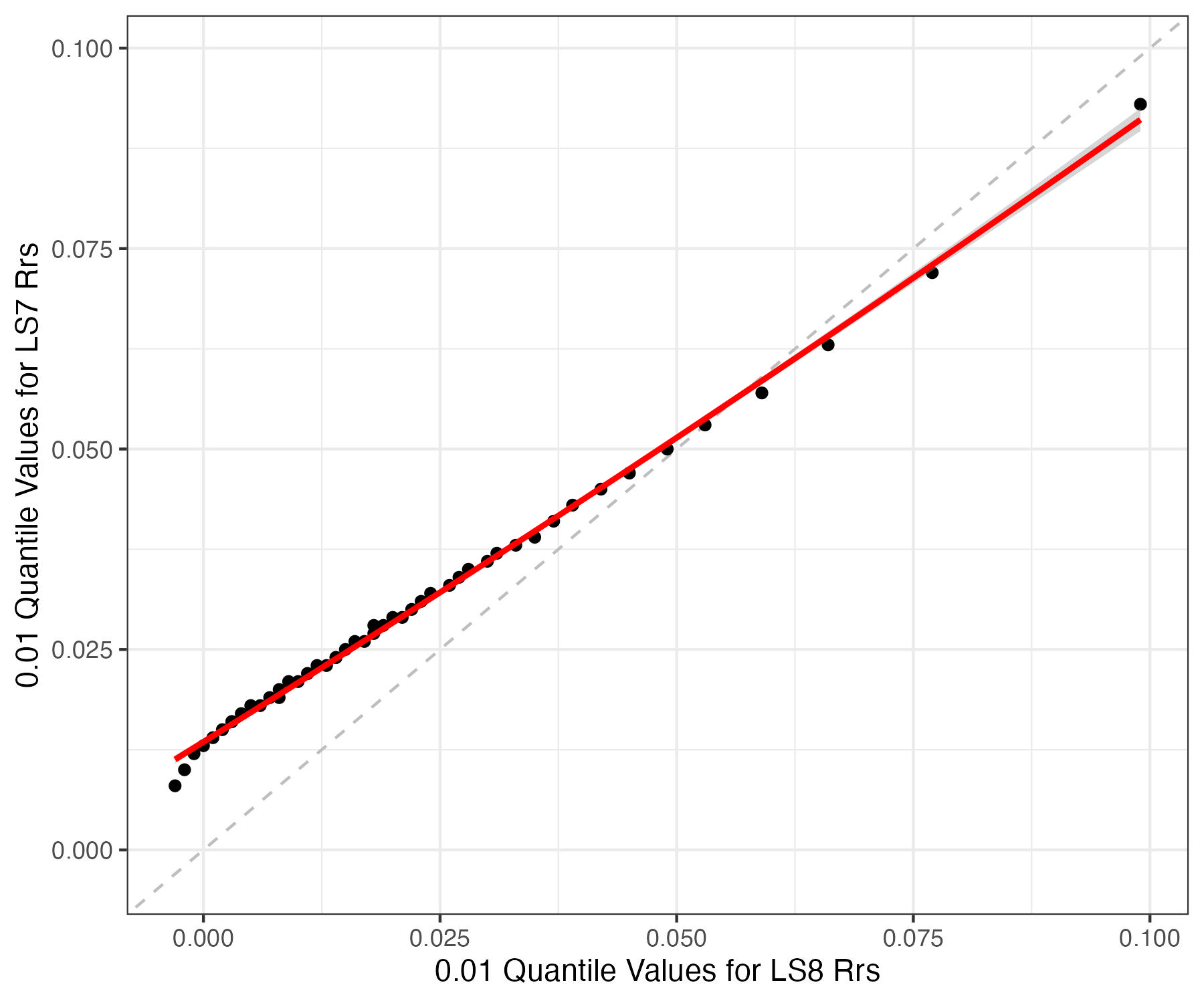
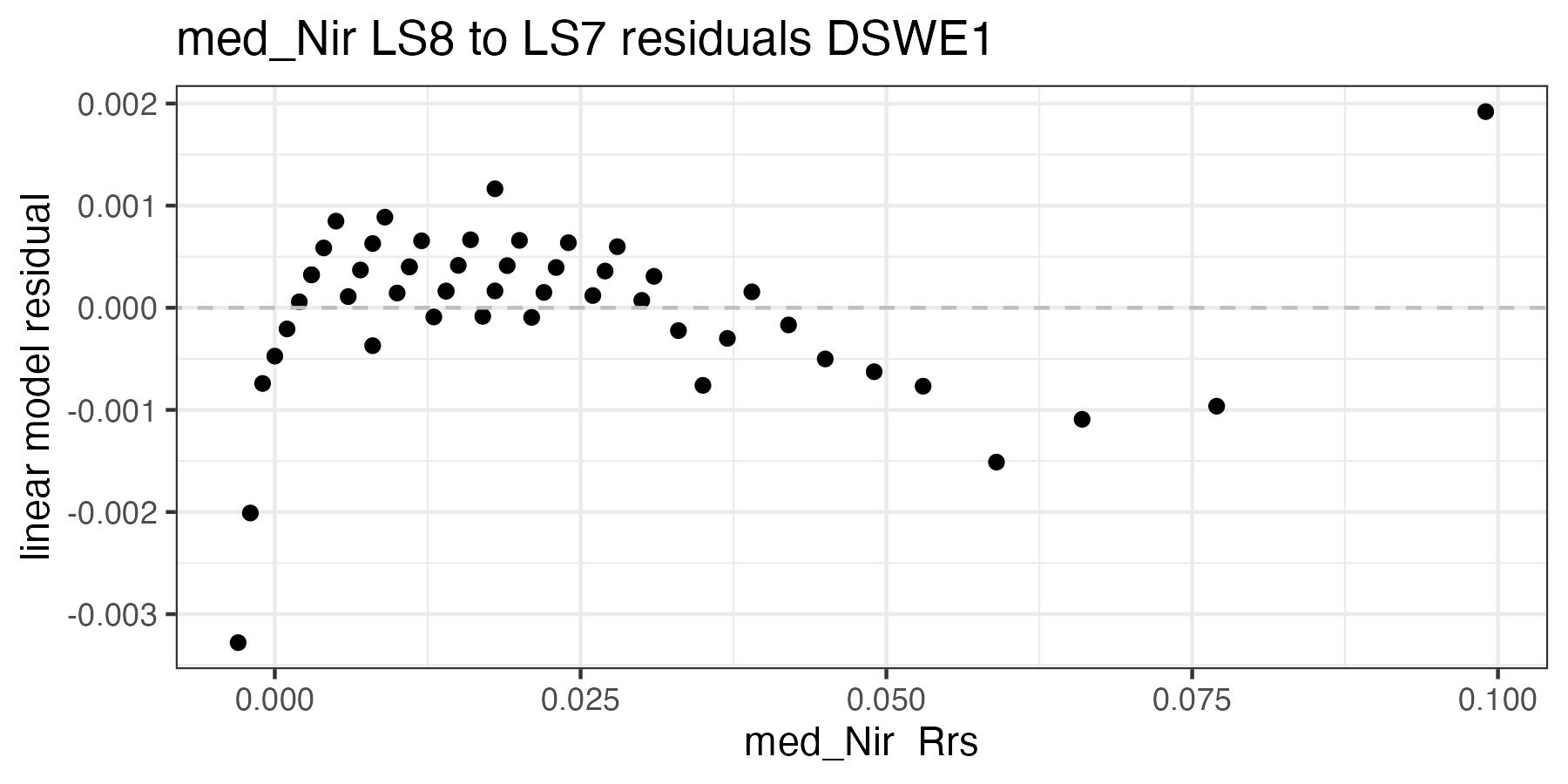
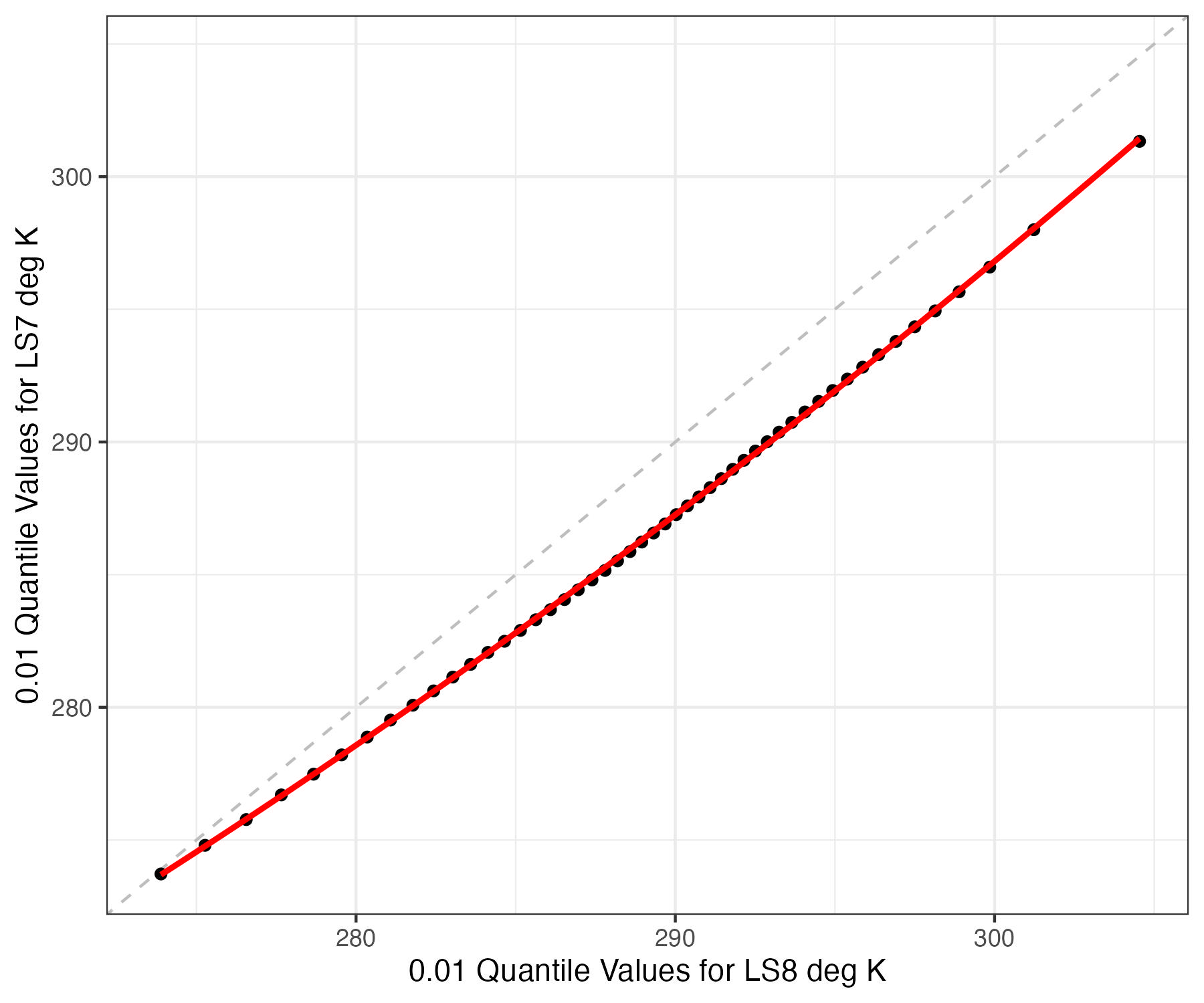
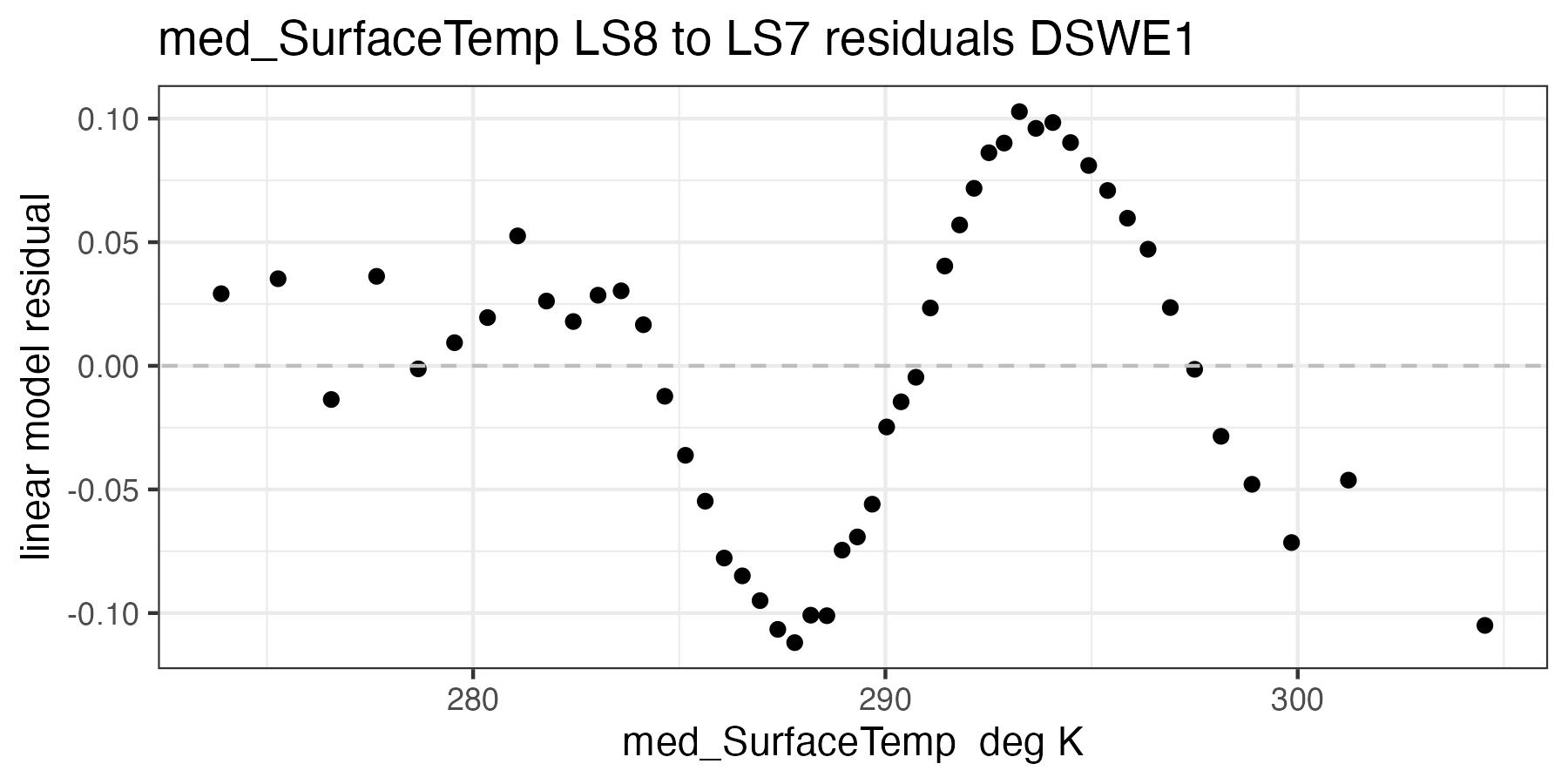
8.5.2 Gardner Correction Landsat 8 to Landsat 7
For each of the handoff figures below, the red line is the second order polynomial regression and the grey dashed line is the 1:1 line. Coefficients for the second order polynomial regression are provided in Table 8.5. Color of dots represents the density of points in at a given x, y location. In the residual plots, the grey dashed line is a 0 intercept, 0 slope line visual aide.
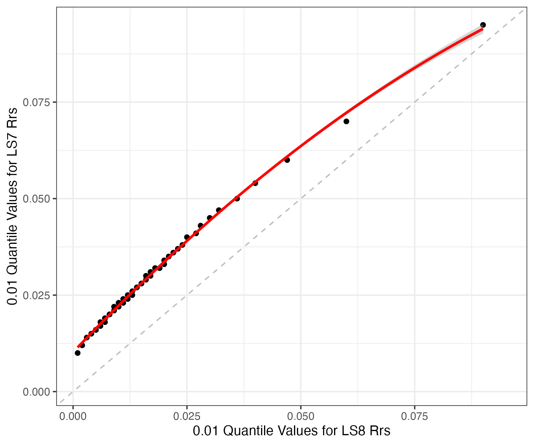
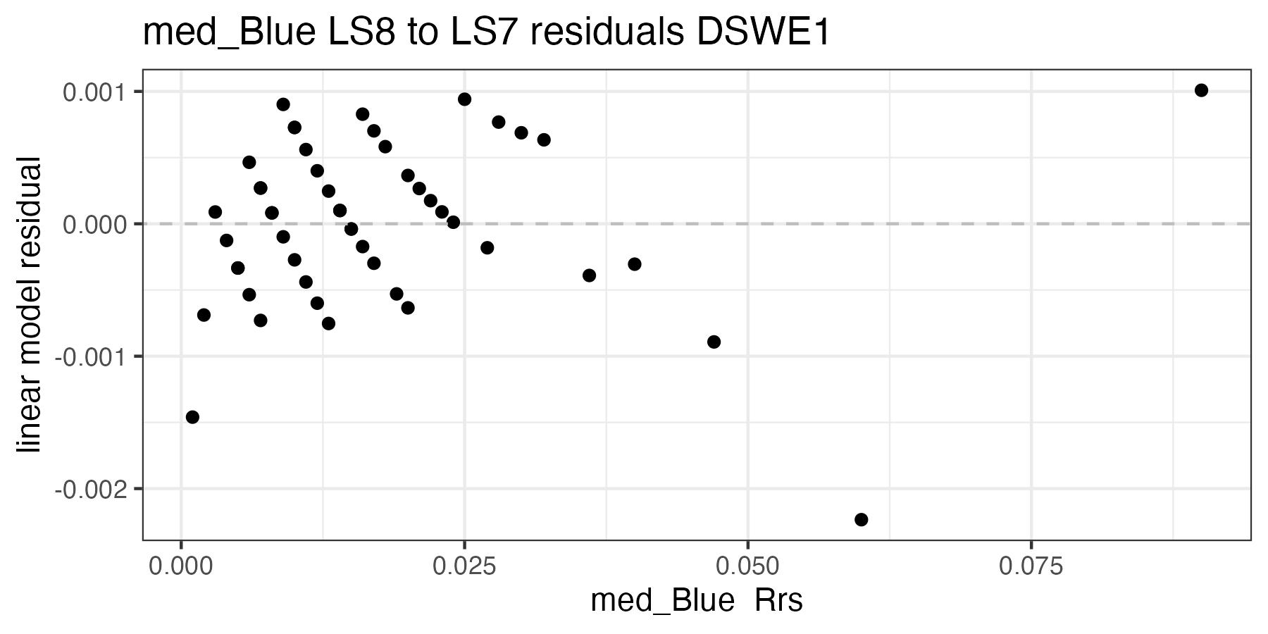
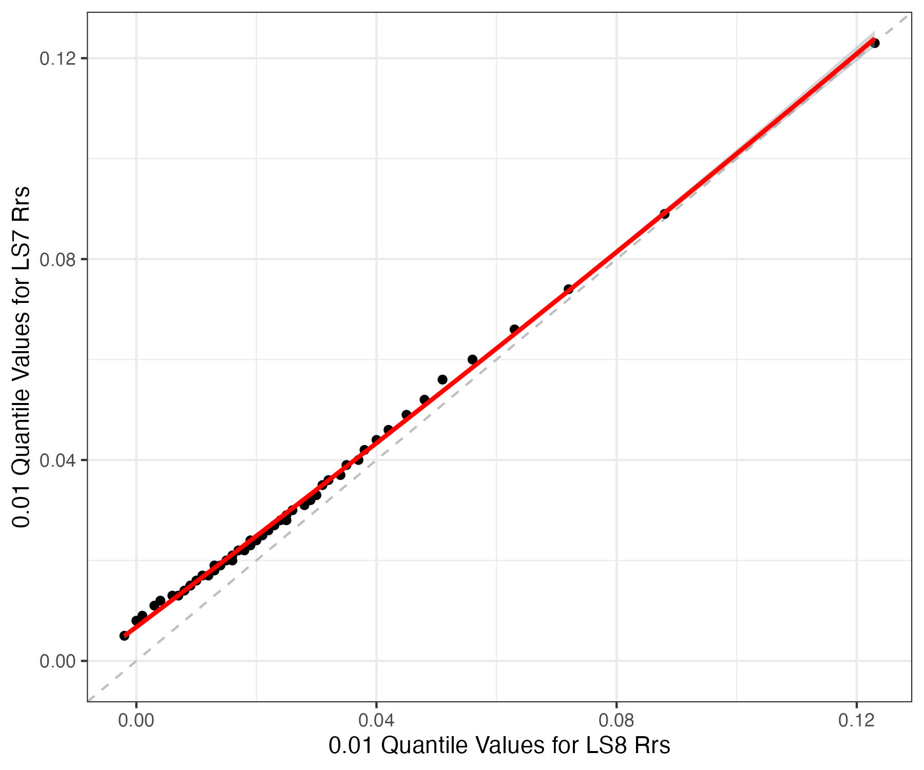
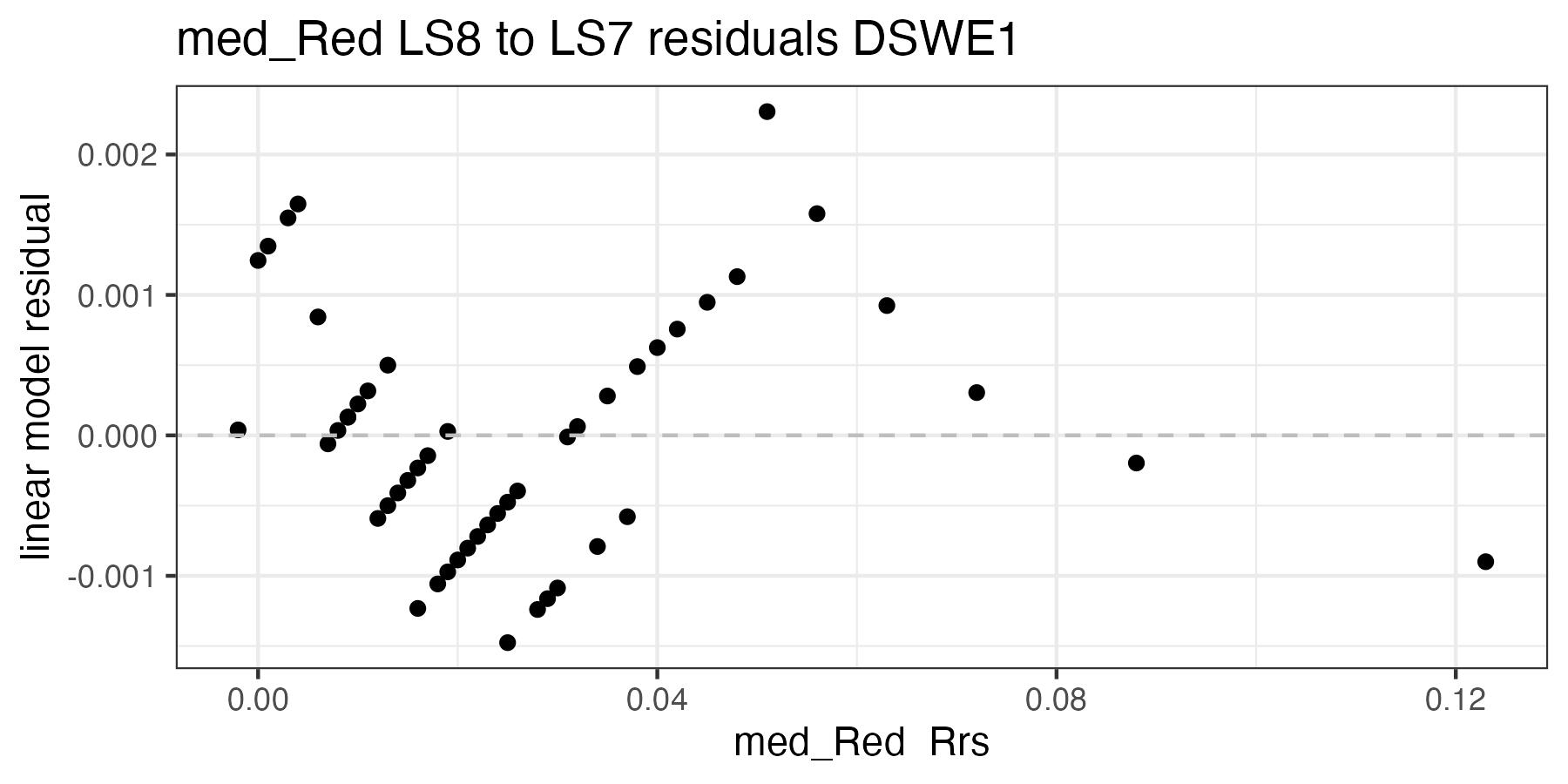
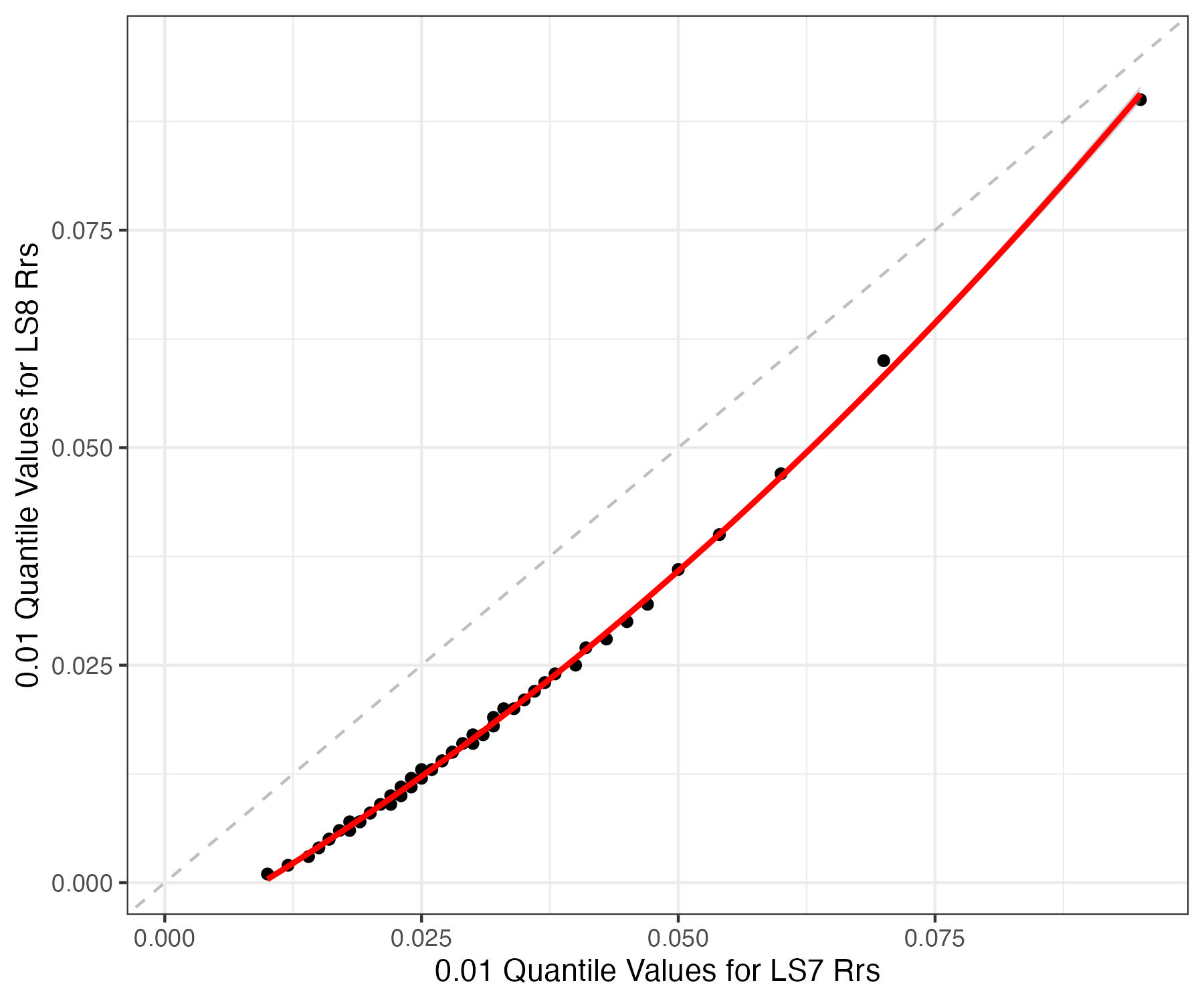
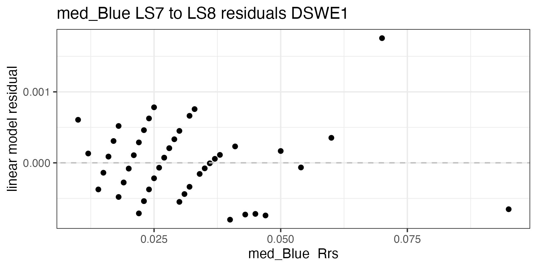
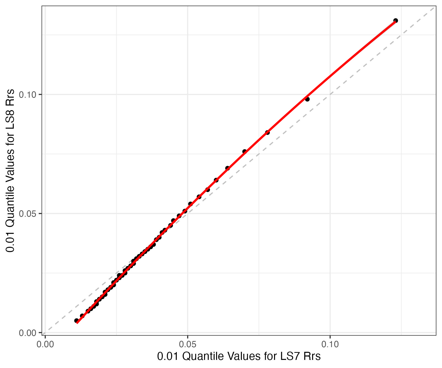
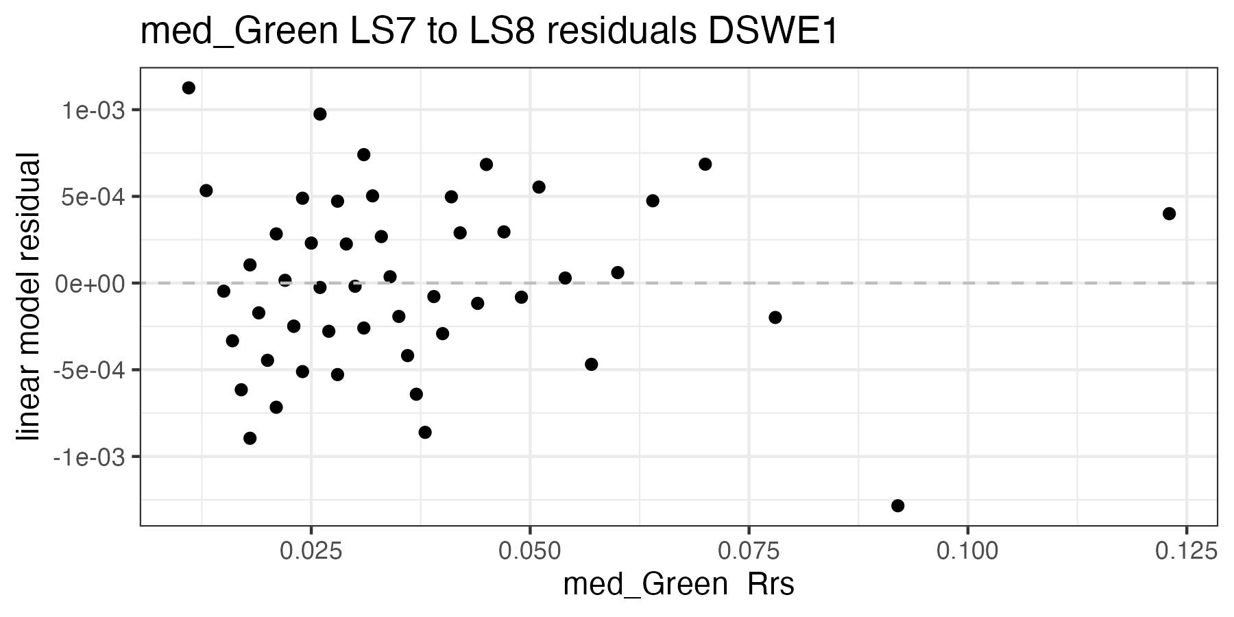
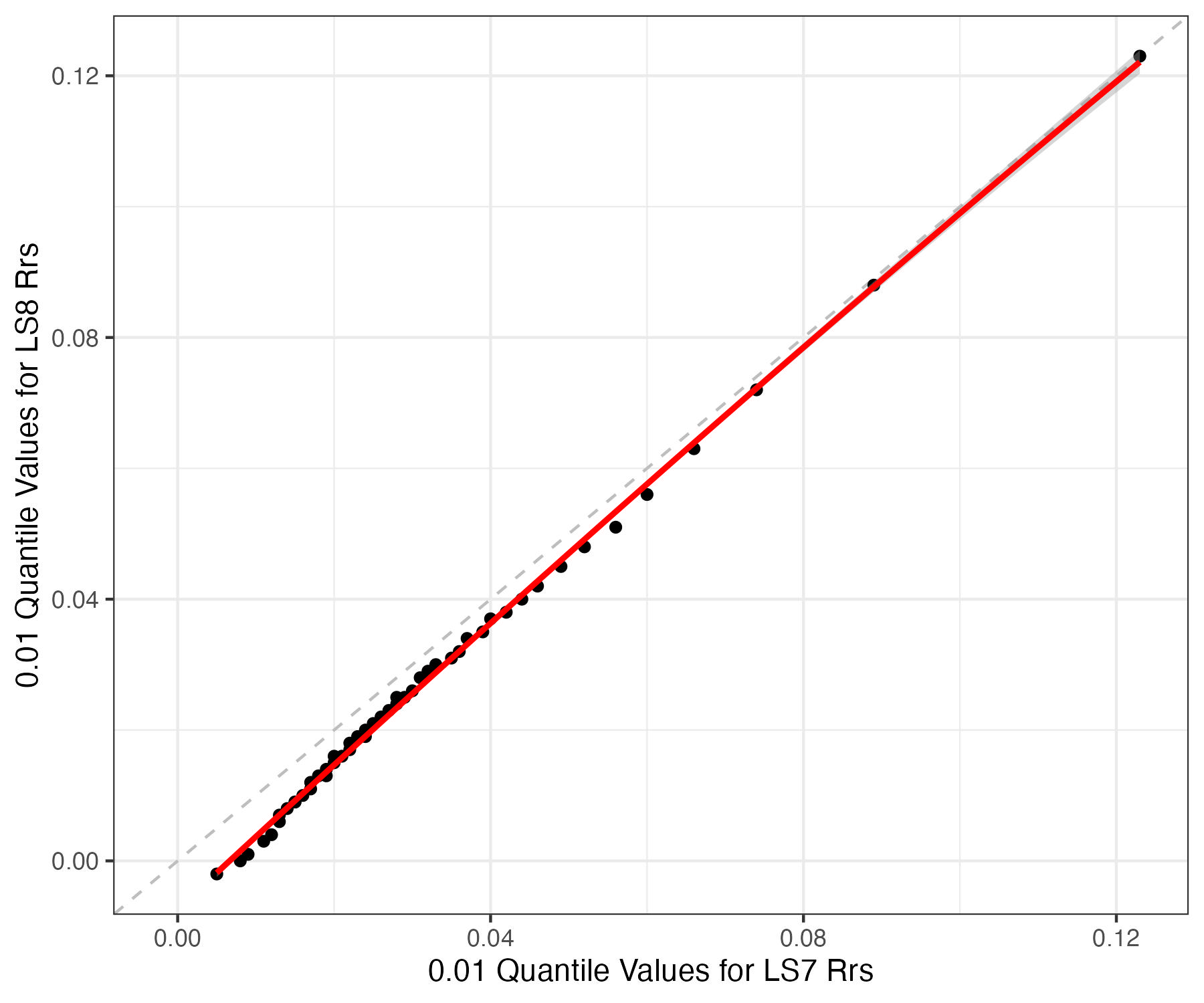
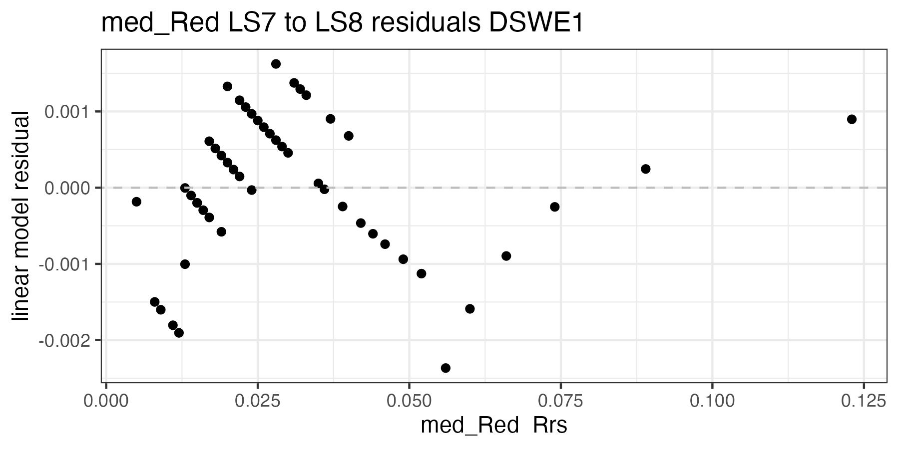
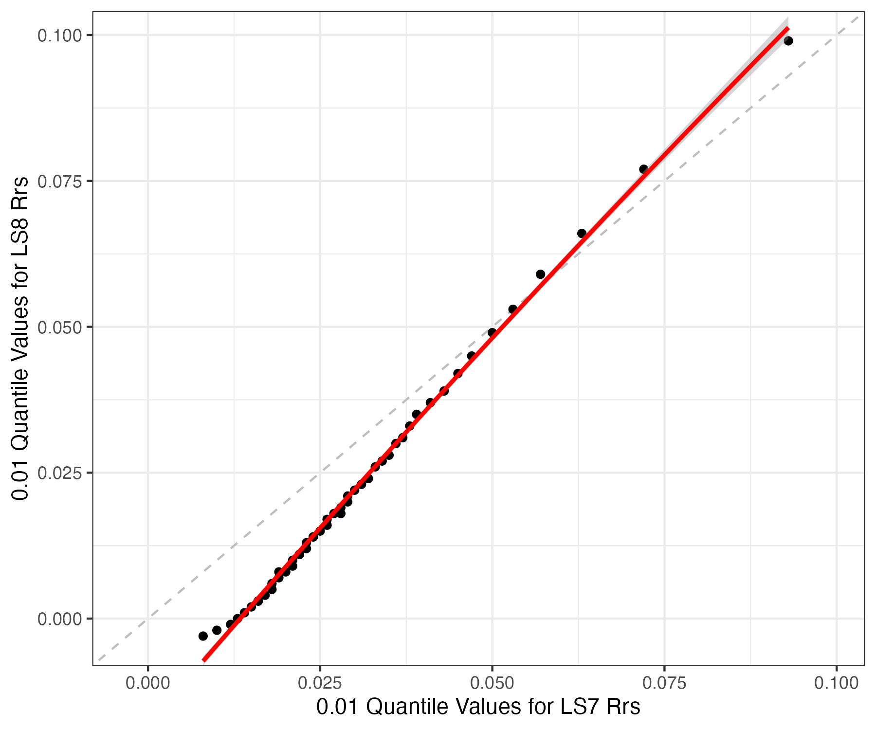
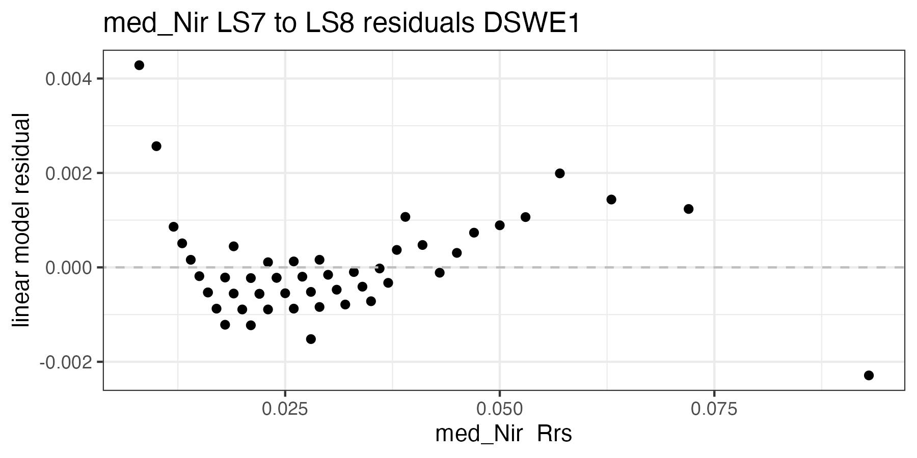
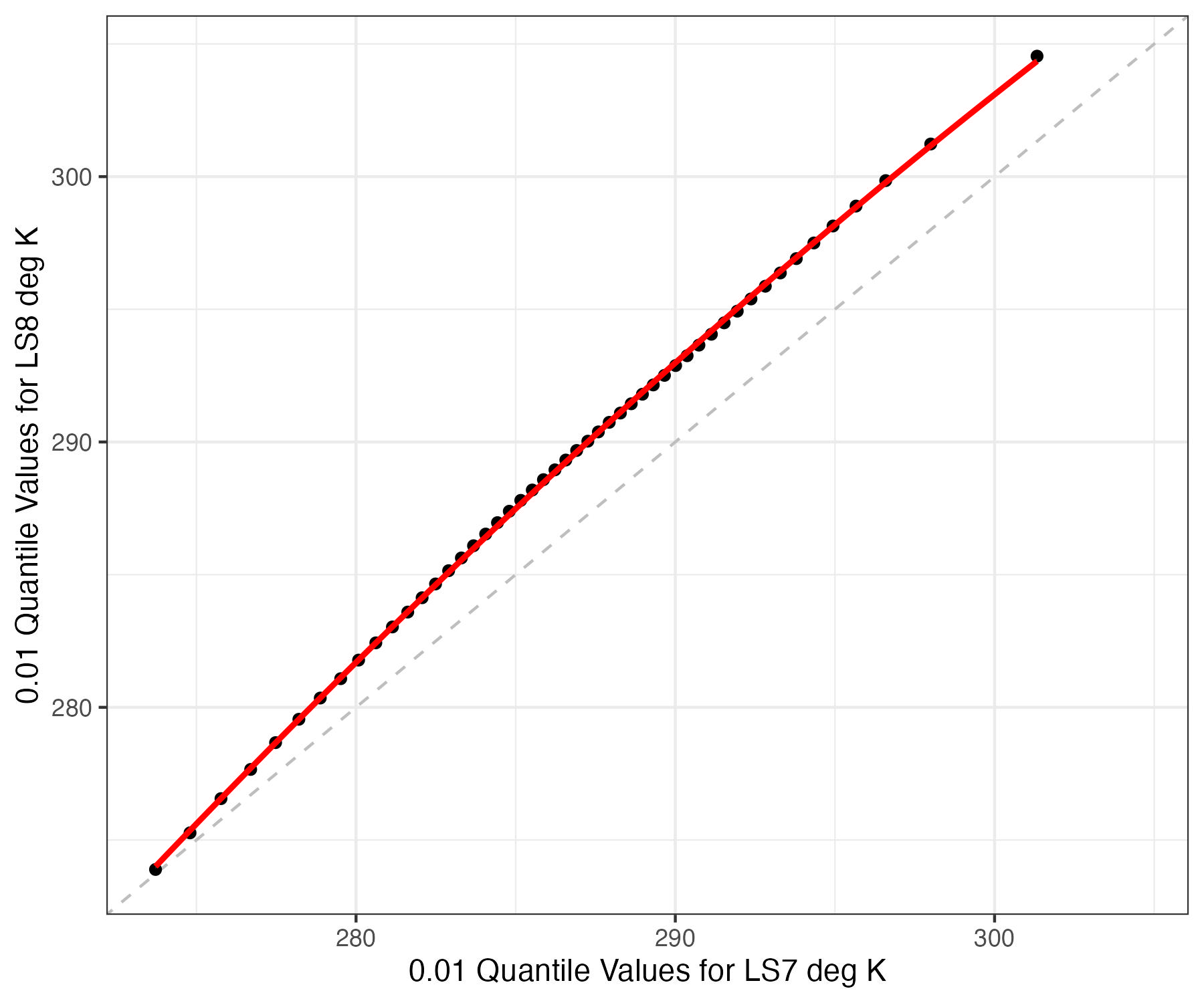
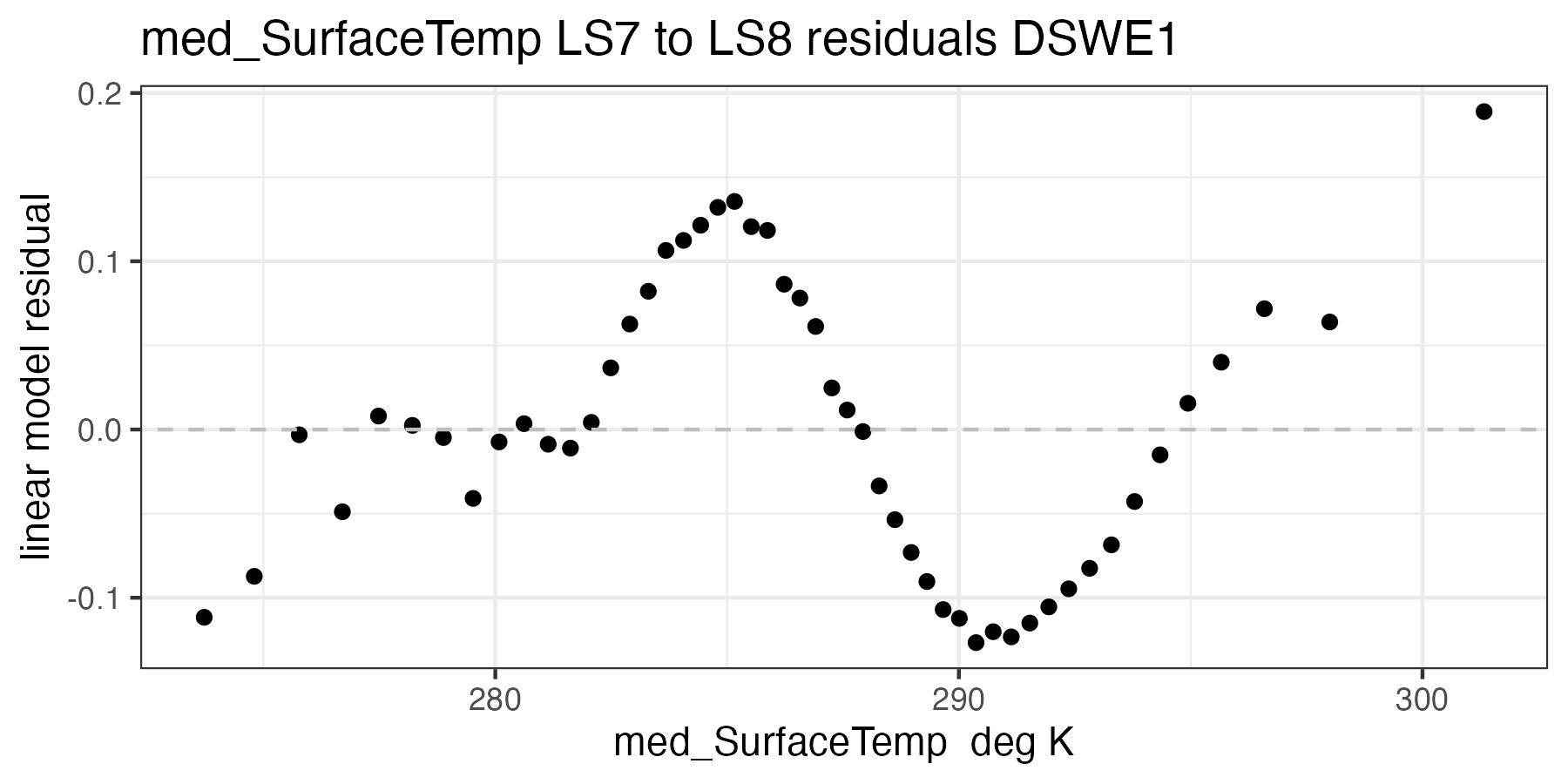
8.5.3 Gardner Correction Landsat 7 to Landsat 8
For each of the handoff figures below, the red line is the second order polynomial regression and the grey dashed line is the 1:1 line. Coefficients for the second order polynomial regression are provided in Table 8.6. Color of dots represents the density of points in at a given x, y location. In the residual plots, the grey dashed line is a 0 intercept, 0 slope line visual aide.